Monte Carlo Simulation

Real-life is full of uncertainties. But, that does not mean that we have to leave everything to fate. There is a way to estimate uncertainties. And that is what Monte Carlo Simulation does. To understand Monte Carlo Simulation, first, let's talk about Random Variables. 

What is a Random Variable?

You know that,

Profit = Revenue - Expense

If you want to look back at your past year, yes, you know the value of revenue and expense from the past year. You can plug in those numbers to the given equation and get a value for Profit, which is also a calculated and known number.

But, when you want to predict your future, you do not know what will be your expense and what will be your revenue. So, you cannot calculate your future profit directly.

You may think of a way to estimate the range of possible values of profit like this:

If your Revenue will be 100$, and the Expense will be 20$, then your profit will be 80$.
If your Revenue will be 200$, and your Expense will be 30$, your profit will be 170$.
.........
An unlimited number of statements can be drawn from the above equation. No, it is not a nice way. There can be an unlimited number of combinations that are not possible to manage.

But, say, you can guess a probability distribution of your expense and revenue (based on your experience and history), then, you should be able to estimate your profit, in terms of a probability distribution.

So, your refined formula for calculating profit should become:

Probability Distribution of Profit = Probability Distribution of Revenue - Probability Distribution of Expense

Now, the question is, how can you deduct one probability distribution from another. A probability distribution is not a single number that you can simply type into your calculator and hit the big PLUS button or the minus button.

The answer is "Monte Carlo Simulation". Using Monte Carlo Simulation, you can get the value of "Profit" as a Random Variable when your Revenue and Expenses are random variables.

Monte Carlo Simulation is a technique that performs random sampling to achieve such a goal. So, let's clarify what Random Sampling is.

Random Sampling

Think about this probability wheel or a roulette.

If you spin this roulette and stop, what do you expect to get on average? "Red" or "Blue"? You can expect that, out of 4 times, 3 times you may get "Red" and 1 time you can get "Blue", right? Because red covers 75% of the disc and blue covers 25% of the disc. In another word, "red" and "blue" follows a probability distribution, as red -> 0.75, blue -> 0.25. Random Sampling is a sampling technique, where a probability wheel is created according to the probability distribution of various numbers and taken a sample from the probability wheel.

For example, say you have a probability distribution like this:

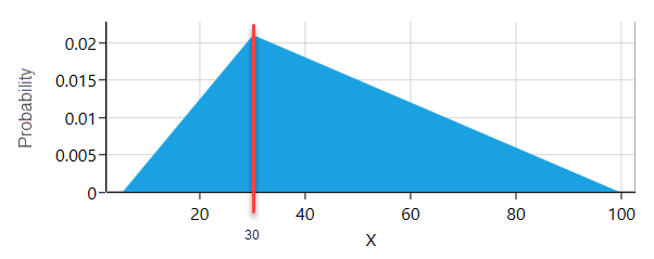
So, if you want to get a random sample from this probability distribution, you can create a probability wheel where each value or outcome will represent a pie in that wheel and the area of that pie will be proportional to the probability of that outcome, which you will get from the probability distribution. Notice that the probability of 30 is 0.02 in the given triangular probability distribution. So, there will be a pie representing the value of 30, in your probability wheel and that pie will cover 2% of the wheel area. Once you create such a probability wheel, if you spin and stop 100 times, you can expect 2 times, the pie for number 30 will show up. For every probability distribution, there is a mathematical formula available for such a hypothetical probability wheel. Most of them are complex to calculate. But, when you use the SpiceLogic Rational Will or Decision Tree Software, the software will take care of such calculation, while you can focus on the big picture of your decision problem.

How Monte Carlo Simulation can evaluate the function of Random Variables.

Ok, so far, you understood what Random Variable and Random sampling are. Say, you are a project manager of a project where you need to predict the profit of your next project, where you have evaluated the probability distribution of Revenue and Cost from various statistical data.

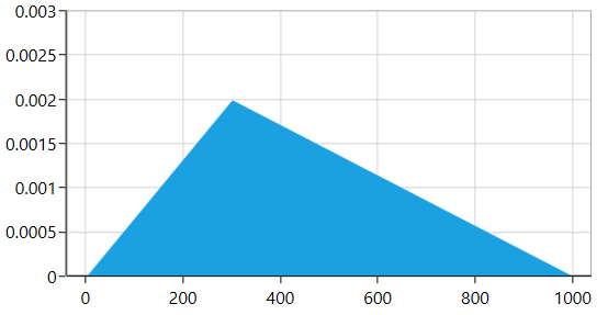
Say, your Revenue follows a Probability Distribution (Normal Distribution) as shown below.

And Expense follows a probability Distribution (Triangular Probability Distribution) as shown below.

As we already mentioned, if you think of creating many combinations like:

Combination 1: Revenue is 500$, Expense is 300$
Combination 2: Revenue is 501$, Expense is 301$
….
.....
You will be overwhelmed. You cannot manage to get all these combinations like this way, right?

Here 'Monte Carlo Simulation' comes to the rescue. What you need to do is, take a random sample from the Revenue probability distribution. Say, you got 500$. Then, take a random sample from the Expense probability distribution. Say, you got 200$. So, for the first round of sampling, your total profit is 500$ - 200$= 300$.

Now, take another random sample, say, it is 400$ for Revenue, and 300$ for Expense. So, for the second round of sampling, your profit will be 100$

Keep doing for many many times, (usually 10,000 times or more).

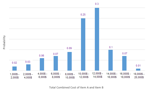
After taking thousands of samples, you can organize the sample data to a histogram, where, the X-axis indicates a range of profit, and the Y-axis represents the number of random samples fell into that profit range.

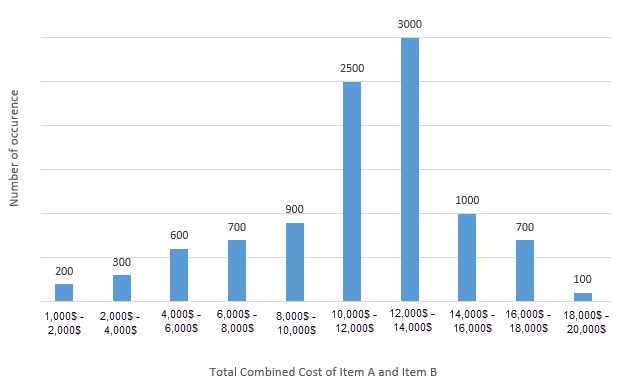
From the above chart, you can understand that, out of 10,000 samples, 200 of them fell into the profit between 1,000$ to 2,000$. 300 of them fell into the range of 2,000$ to 4,000$ and so on.

As we get the total count for each profit range, we can get the probability of a range as :
sample count in a range/total samples (which is 10,000).

So, the probability of the profit range 1,000$ to 2,000$ is = 200/10,000 = 0.02. Finally, we can get the probability distribution of profit, like this:

This way of finding an ultimate probability distribution of a dependent random variable is called "Monte Carlo Simulation".

Step by Step Modeling Example

Ok, let's model the discussed random function Profit = Revenue - Expense, where both Revenue and Expenses are random variables.

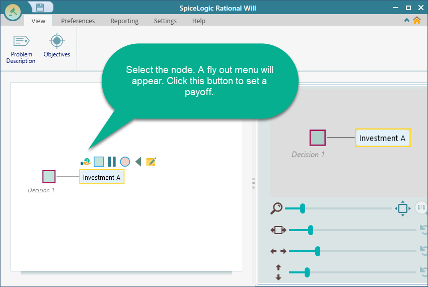
Start the Decision Tree analyzer and model a simple decision tree like this, where there are just one Decision Node and one action.

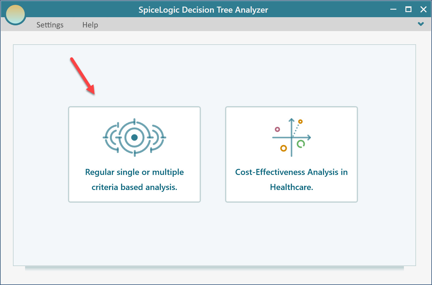
Once you click the "Pay off" button first time in the project, you will be asked if you want to use a regular single/multiple criteria analysis or Cost-Effectiveness analysis. Choose the first option. 

Then you will be presented with the following screen. Select "Maximize" and enter "Revenue" as shown below.  

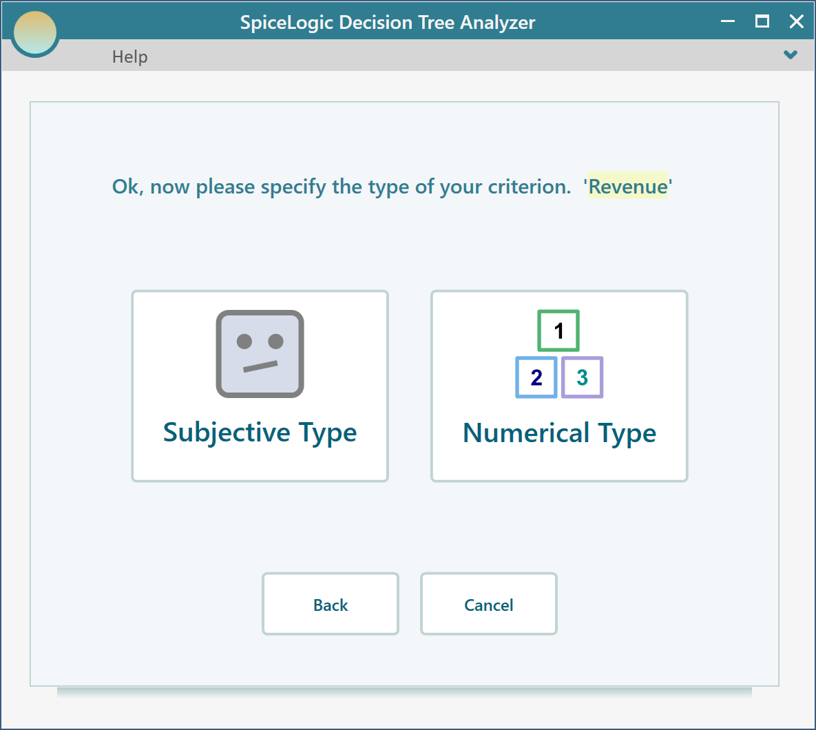
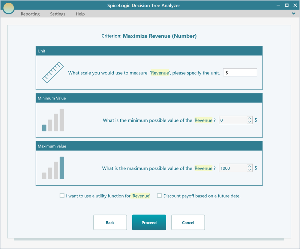
Then click the "Proceed" button. You will be asked about the type of criterion. Select "Numerical Type".

Then, you will be asked to enter the Minimum value, Maximum value, and a unit. Let's use $ as the unit, the minimum value is 0, and the maximum value is 1000$.

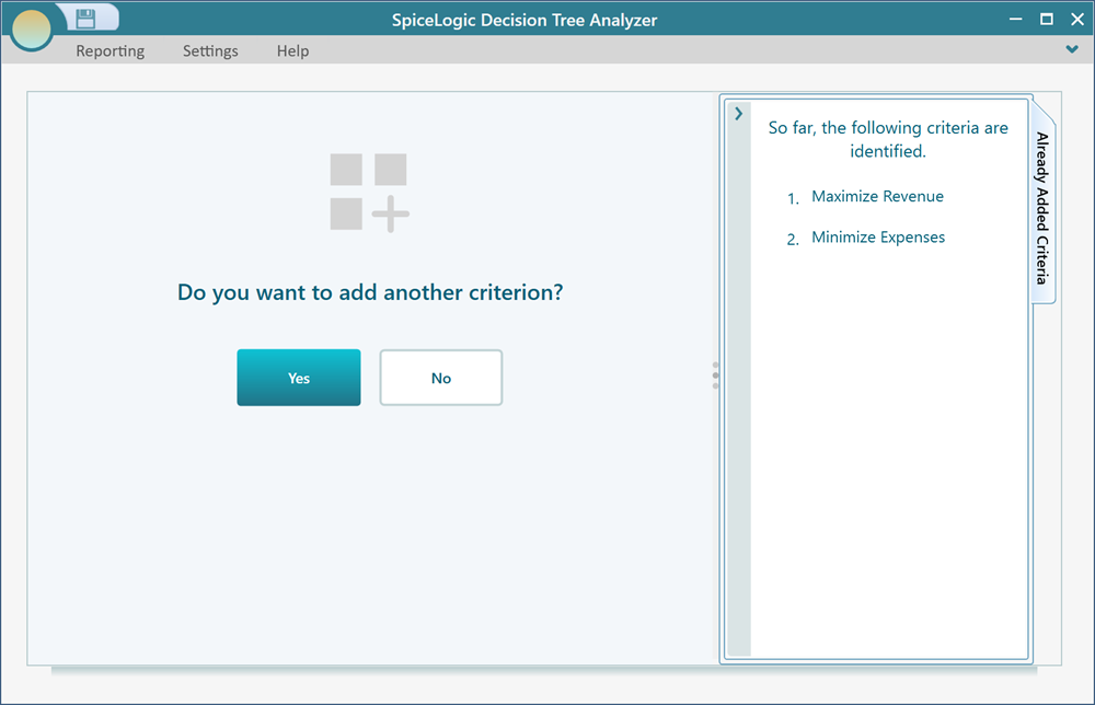
Then click the button "Proceed". You will be asked if you have another criterion to add. Click Yes. And then, in the same way, create a numerical objective "Minimize Expenses".

Once you are done adding the second criterion, answer "No" when you are asked to add another criterion.

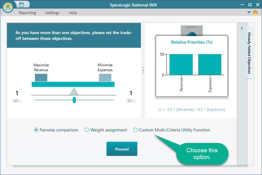
Now, you will be asked to set up a trade-off between the criteria, to form a multi-criteria utility function. You have various choices like Pairwise comparison, custom expression, etc. Let's choose the Custom Multi-Criteria Utility Function from the following screen.

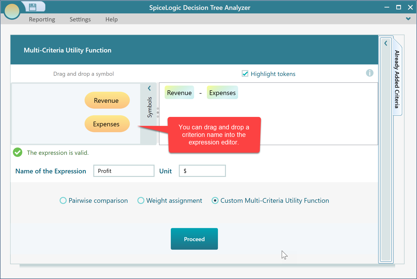
Once you click the box "Custom Multi-Criteria Utility Function", a rich math-based equation editor will appear. In this expression editor, you can use a rich math-based function, like sqrt([Revenue] - ln([Expenses]) etc. Our expression is very simple. Just [Revenue] - [Expenses], so keep the expression as shown here.

Then, click the "Proceed" button. You will be taken back to the Decision Tree. The payoff editor will be shown. You may enter simple values for Revenue as 500$ and Expenses as 300$. You will see that the node shows the value as 300$, which makes sense, as according to our custom expression, Revenue - Expenses = 500 - 200 = 300.

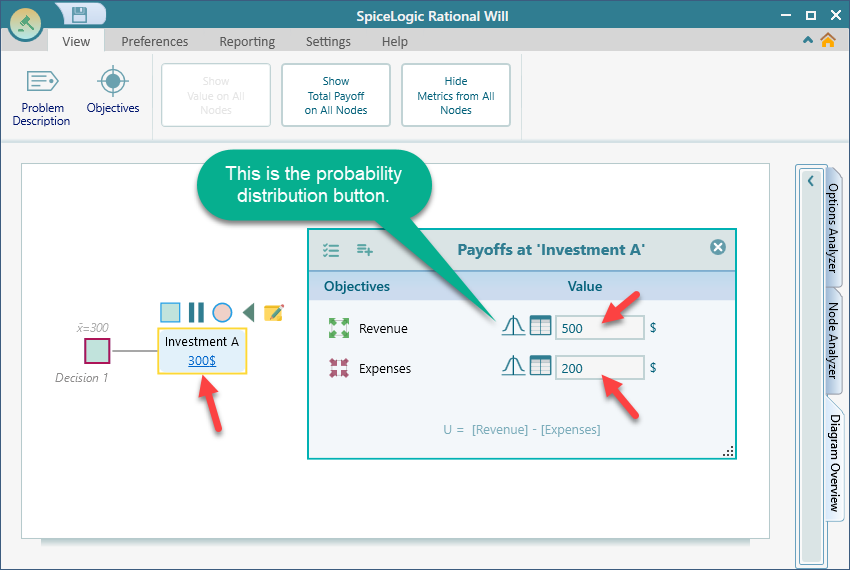
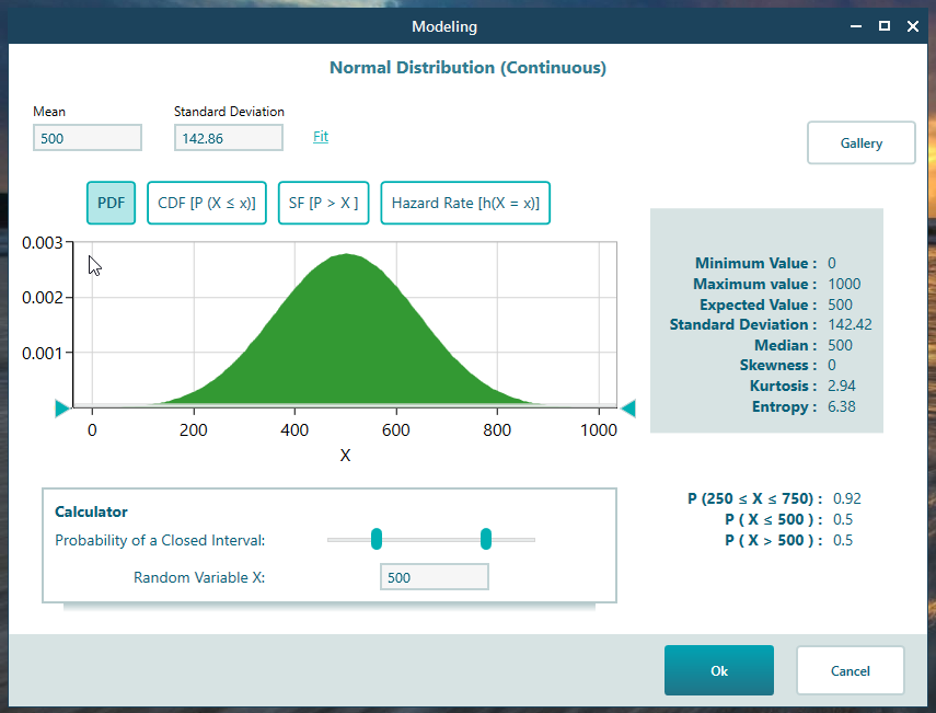
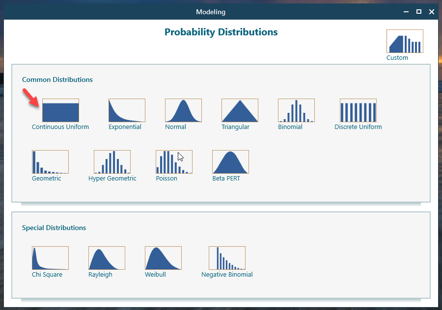
Ok, now, let's use a probability distribution "Revenue". Click the probability distribution icon in the Revenue row as shown in the above screenshot. The probability distribution window will show up. Then click the "Continuous Uniform" distribution as shown below.

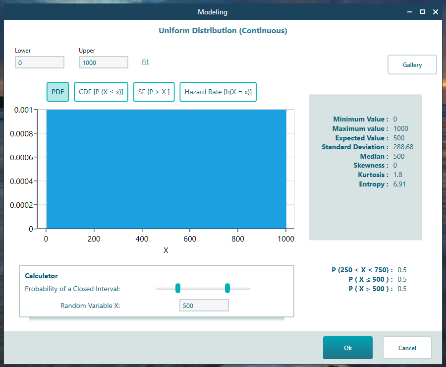
We just left the default setup and clicked the OK button.

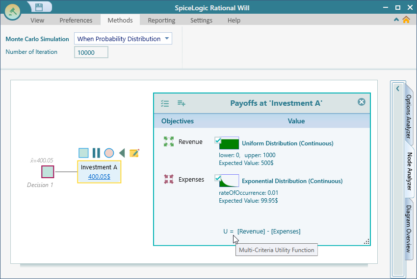
Same way, set another probability distribution for the Expense criteria. This time, choose "Exponential" distribution from the probability distribution gallery. Keep the default setup and proceed, as shown below.

Finally, the payoff editor in the Decision Tree diagram will look like this.

Alright. now, let's see the magic. Open the Options Analyzer and notice the Risk Profile chart carousel. 

Keep the action node "Investment A" selected in the diagram and expand the tab "Node Analyzer". Also, in the Ribbon, you will see a number box for "Number of Iteration" under "Monte Carlo Simulation". Set that to 10,000. A higher number of iterations gives a better result. 

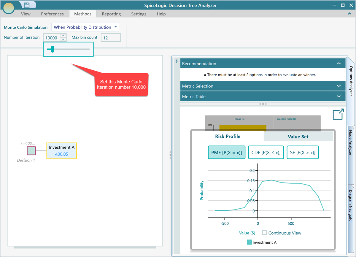
Cool. Now, we can see a probability distribution of our Random Variable "Profit" which is equal to the Random Variable "Revenue" - Random Variable "Expenses". The decision tree analyzer software has performed a Monte Carlo simulation for us and produced this probability distribution. This probability distribution chart is the result of a deduction of two probability distributions, as defined in our custom expression editor.

If you add another action node to the Decision Node, then based on Monte Carlo simulation, the action that gives a higher expected value, can be chosen as an optimum action.

 In the ribbon, there is another number input called "Max bin count". The bin count indicates, how many bins or segments we should use to distribute the simulation results. If you use a high number of bins, then the simulation result will look evenly distributed among all bins which may not be very useful. If you use a very low number of bins, you will see the results are highly varied between bins and that may be useful for many analyses. By default, the decision tree software uses 12 bins. Let's change that to 5 bins. See the result.

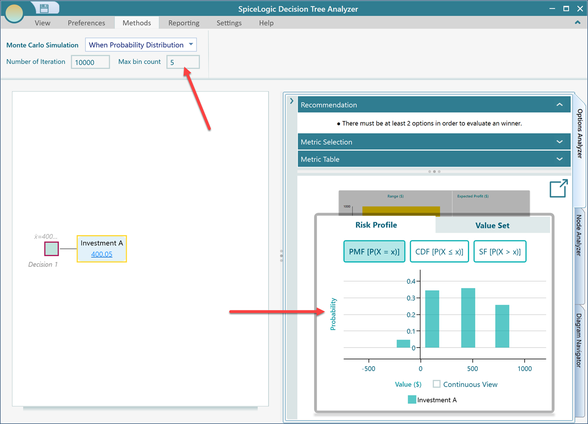
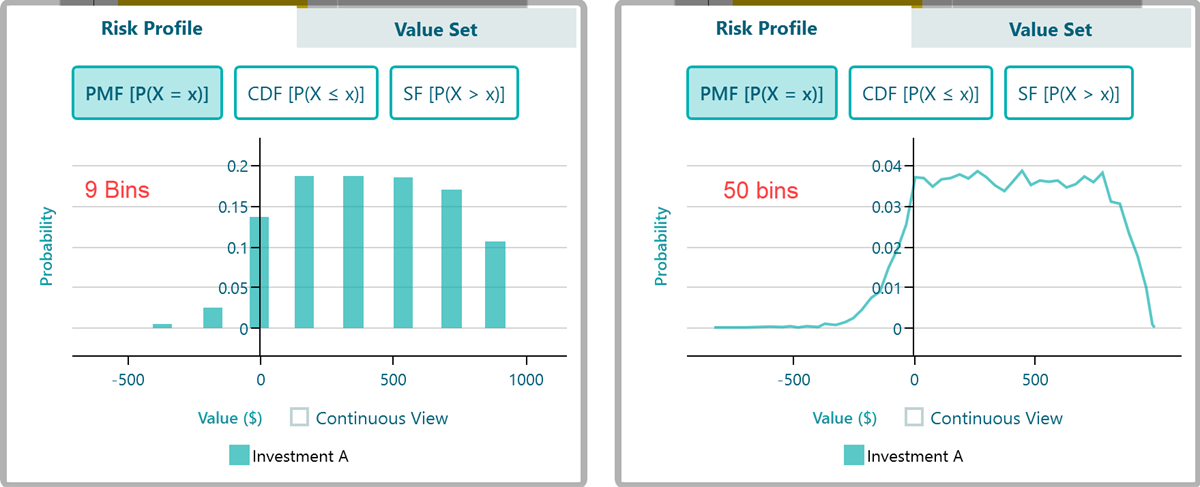
Now, you see, the results are segmented between a few segments. The following screenshot shows the risk profile with 9 bins and 50 bins respectively.

Random Function as a decision tree

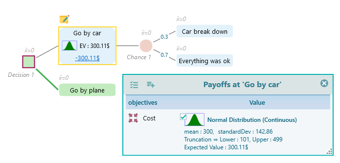
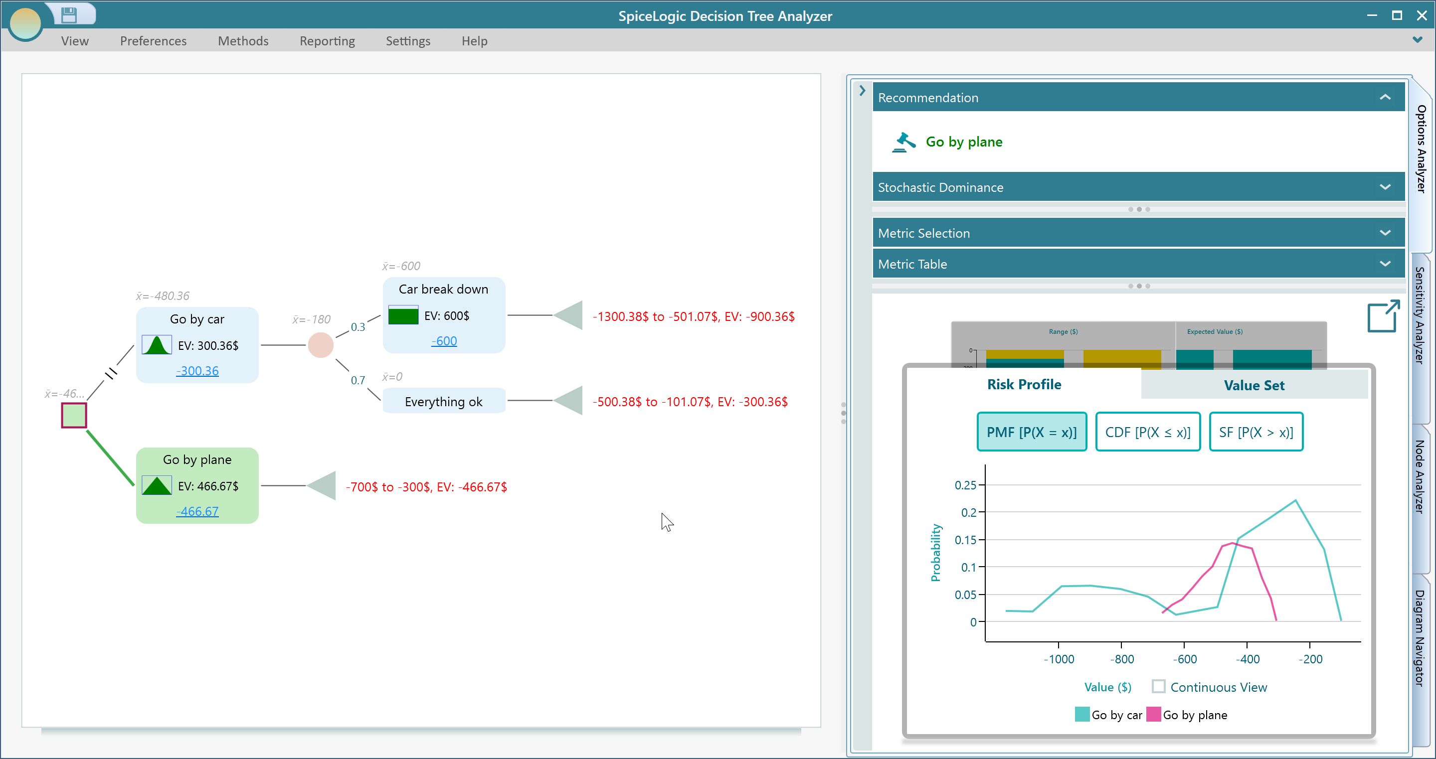
Let's model something for real. Say, you are planning for a vacation where you can go by car or by plane. If you go by car, your car can break down on the road and it may cost a variable amount of money. Also, you know that the cost of a plane ticket does not stay the same. It changes all the time. Assuming that you have learned how to create a decision tree using the Decision Tree software. Let's create a decision tree like this:

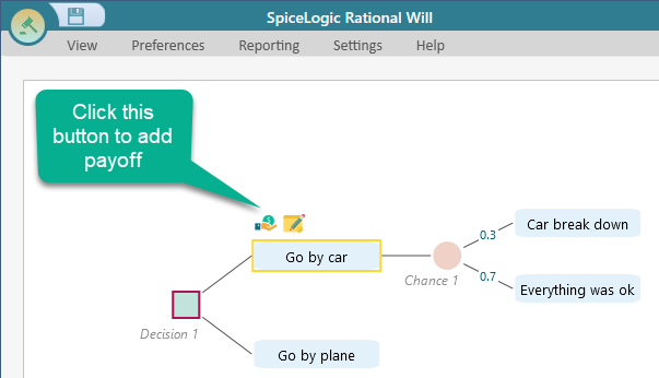
You are assuming that the probability of getting the car breakdown is 0.3. So, set the probability as shown in the above screenshot.

Now, let's create an objective "Minimize Cost". From the flyover menu of the "Go by car", click the "Payoff" button. The objective creation wizard will appear. Create an objective "Minimize Cost" same as before. Chose that as Money type or Number type with unit "$", minimum value 0 and maximum value 1000$ as shown below.

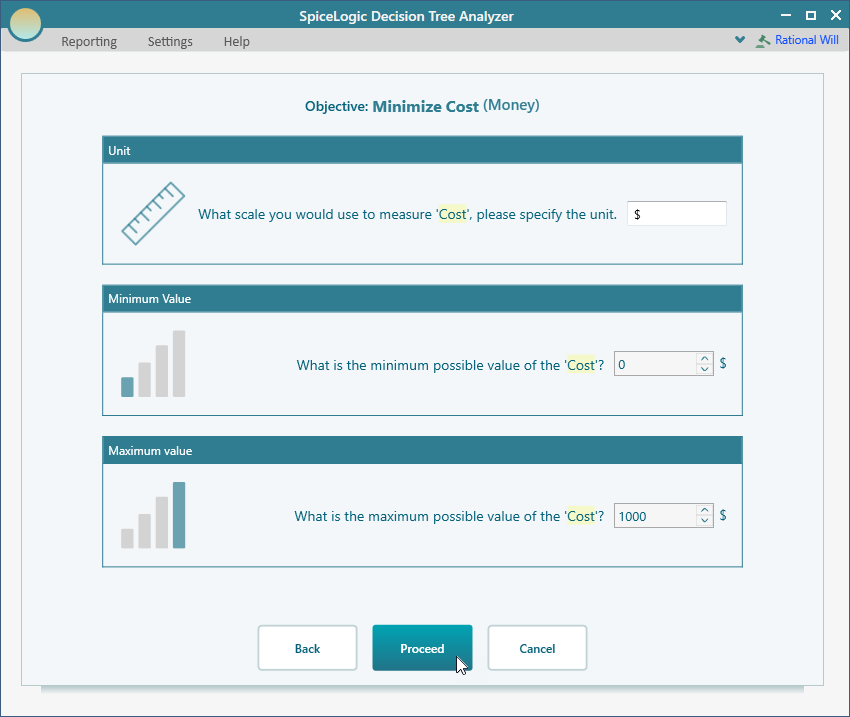
Then, click Proceed. When you will be asked, if there are any more objectives to add, answer 'No', and then, you will be taken to the decision tree, like this.

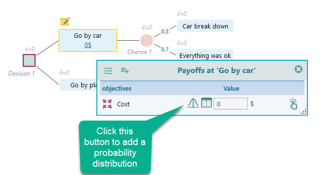
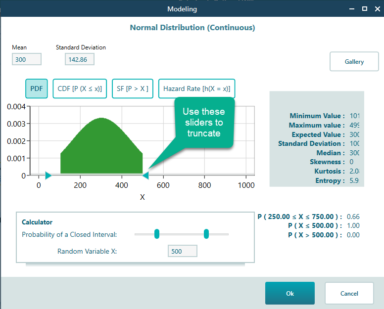
Say, your cost for driving by car, can be anywhere from 100$ to 500$, because, you do not know how much would be the gas prices in various locations, how much food you may need to buy, etc. But, you can guess that most probably the cost will be close to 300$. The probability of the cost '500$' or '100$' is relatively low. Therefore, a normal distribution with a mean of 300$ can suit this scenario, right? Let's click the probability button from the payoff editor, and chose "Normal Distribution" this time.

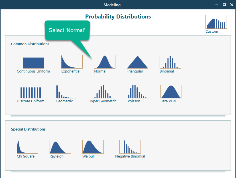
Once you select the normal distribution, you can specify the mean and standard deviation.

\

Click Ok, to accept the modeled probability distribution. The decision tree diagram will look like this.

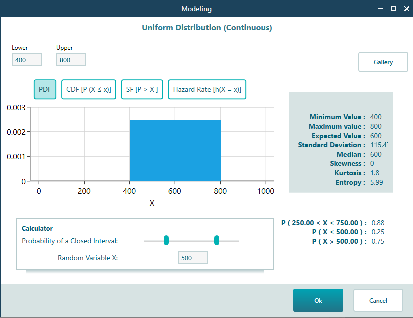
Now, use a probability distribution for a Car break down the cost, which you are thinking, maybe within 400$ to 800$, and you do not have any clue about the most likely value. So, you can use a uniform probability distribution. According to the principle of indifference, if you have no reason to believe that one event will occur more likely than another event, then you can assume the same probability for all possible events. Therefore, according to that principle, as you cannot guess what kind of car breakdown may happen, you may use the continuous uniform distribution where the probability of each input is the same. So, same like the Car cost, attach a Uniform probability distribution that ranges from 400 to 800, like this:

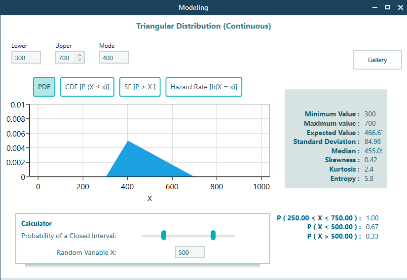
And use another probability distribution for the Plane cost. You are assuming that the most likely value for a plane cost is 400$. But, it can be more or less, perhaps, 300$ to 700$. You may use a Triangular probability distribution or Normal Distribution, whatever you feel confident about. I think a triangular probability distribution may make sense, like this:

So, finally, the decision tree will look like this.

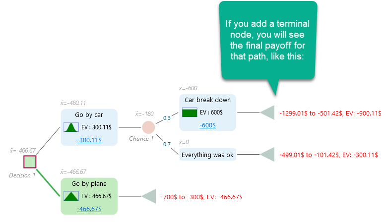
Ok, you have completed the modeling. Now, you can expand the Options analyzer panel to see all the calculated results. And guess what, the Monte Carlo Simulation is already performed for you. Just notice the probability distribution shown in the risk profile panel at the options analyzer, this probability distribution is the result of Monte Carlo Simulation.

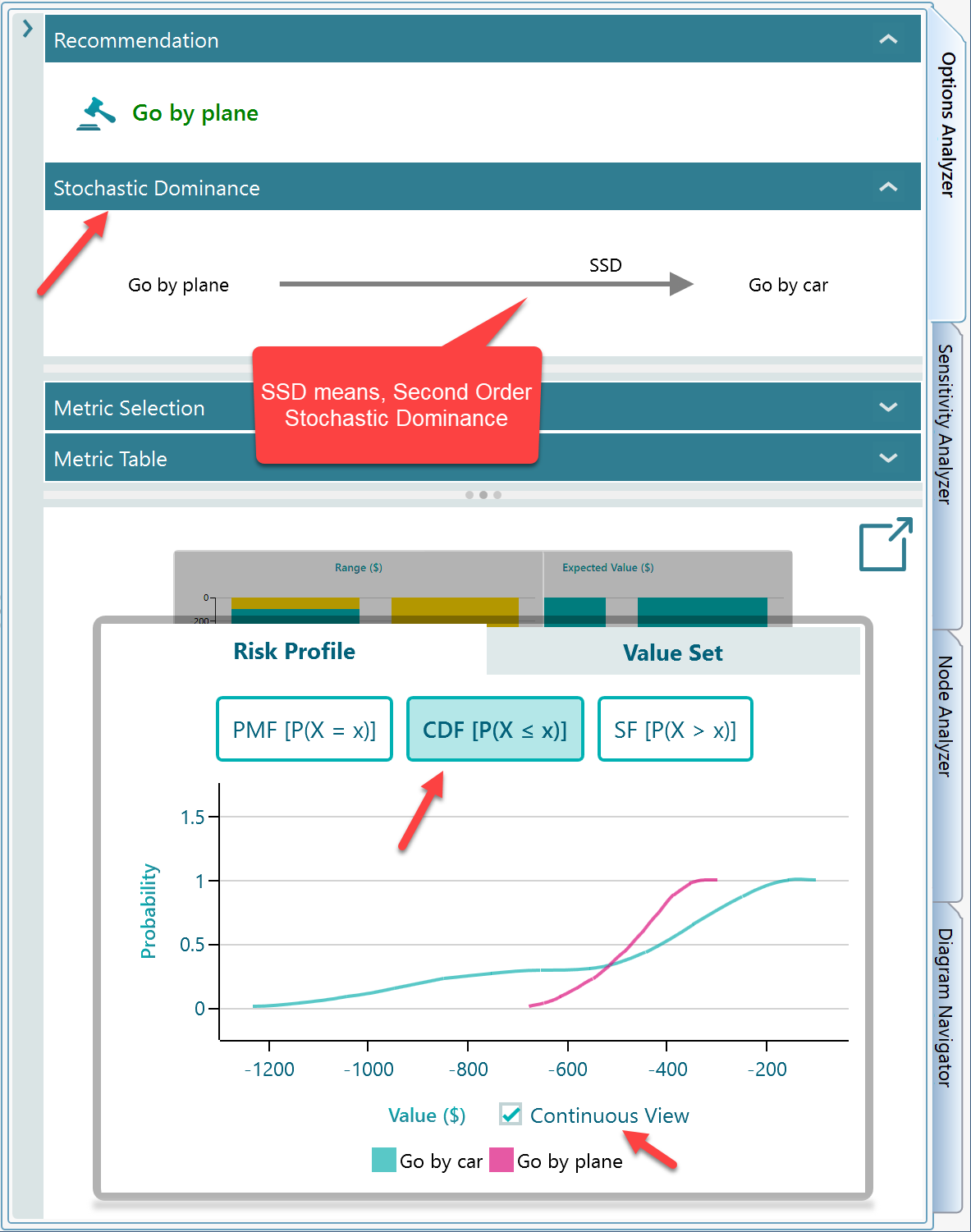
You can resize panels to get a better view of the results. As shown below. (Notice that, Stochastic Dominance is also calculated from the risk profile). Expand the Stochastic Dominance Panel to see the dominance diagram.

In the Risk Profile chart, select CDF view to see the Cumulative Distribution Function which is a better view for understanding Stochastic Dominance. Also, check the Continuous View checkbox as shown in the following screenshot which gives a better graphical view.

Explanation of the Result

Ok, the SpiceLogic Rational Will or Decision Tree Software has generated the Probability Distribution (In the Risk Profile panel). But How? The software, created thousands of random samples as follows:

1. A random sample is taken from the probability distribution of the "Go by Car" node. Say, that value is "p". Then, applying the probability wheel, from the chance node, an event node is selected based on the probabilities of the event node (i.e. 0.3 for the car break down). If the "Car breaks down" node was selected from the probability wheel of the chance node, a random sample is taken from the probability distribution of the "Car break down" cost. Say, that value is "q".

So, in the first round, the total cost is calculated as "p + q".

2. The same process continued thousands of times and a lot of outcomes were calculated. The software decides to show 100 groups of data. Therefore, it creates a group interval for the total outcome such that, there will be a maximum of 100 groups. As you can see from the above screenshot, where the tooltip shows the group "-932.36 to -920.36" is a group of the outcome, and the probability of that group is 0.01.

Options for Monte Carlo Simulation

By default, the Monte Carlo Simulation option is turned on for any scenario when a Probability Distribution is used.

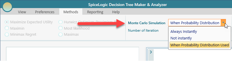
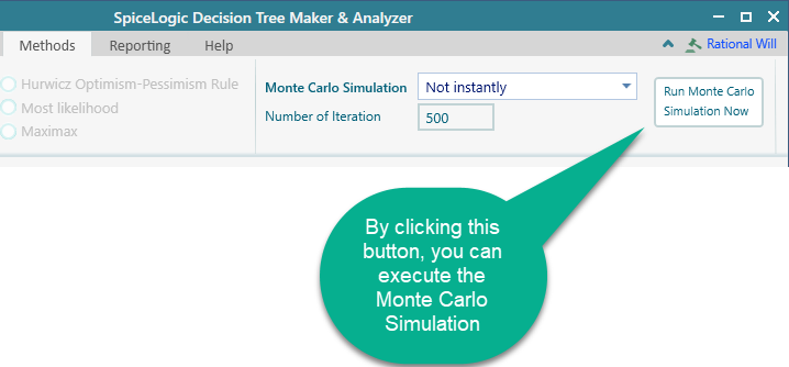
You can turn off that behavior completely by setting the drop-down box selection to "Not Instantly" as you can see in the above screenshot. If you set it to "Not Instantly", then, you will see a button to Execute the Monte Carlo Simulation so that you can manually execute the Monte Carlo Simulation whenever you wish.

If you set the option to "Always Instantly", then no matter if Probability Distribution is used or not, if there is at least a chance node in a decision tree, Monte Carlo simulation will be used to generate the Risk Profile.