Exponential Utility Function
What is the Exponential Utility Function?
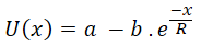
In economics and finance, exponential utility refers to a specific form of the Utility Function. This utility function is mainly used for mapping real-world Monetary gain to perceived value. Formally, the exponential utility is given by:

or 
Where R is the Risk Tolerance. x is the real-world value and u(x) is the utility value or perceived value (the value of an outcome in utils). "a" and "b" are essentially scaling parameters. Decision Tree Software can calculate that parameter based on the Minimum and Maximum possible values in the decision context, which is collected from the user.
If you represent real-world money gain on the X-axis and your level of satisfaction on the Y-axis (in terms of 0 to 1, where 0 means no satisfaction and 1 means the highest satisfaction), then the Exponential Utility function will look like this:
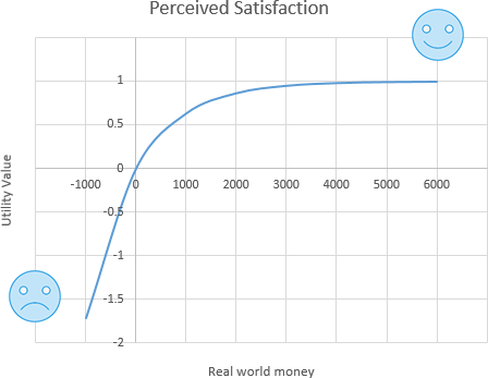
This utility function is concave, and so it can be used to model risk aversion. In such a utility function, R, the Risk tolerance parameter determines how concave the utility function is, which in turn reflects how risk-averse the decision-maker is. In the above chart, we used the Risk Tolerance value (R) = 1000. Greater values of R (Risk Tolerance) make the exponential utility function flatter, while smaller values make it more concave or more risk-averse. When your risk tolerance is infinite, the above function becomes a straight line equation. Thus, if you are less risk-averse, (you can tolerate more risk), you would assess a greater value for R to obtain a flatter utility function. If you are less tolerant of risk, you would assess a smaller R and have a more curved utility function.
The exponential utility function is mainly used to measure the utility of monetary gain where there is a chance of losing money.
From where this utility function comes from
Well, obviously, this function was not derived. The human brain and behavior are more complex than such a modeling function. It is just an idea that, as such function is concave, it can be used to model the behavior of a risk-averse decision-maker. If you look into this utility function ( ), you will notice that, as x increases, U(x) approaches 1, which means the highest utility. The utility of zero in this equation, U(0), is equal to 0. That makes sense as someone who does not get anything, his utility is 0, right?. Then notice that the utility for any negative x (being in debt) is negative, which makes perfect sense too. So, we can whimsically use this utility function, but of course, there is no scientific ground that proves that human attitude perfectly follows this utility function.
How can the Risk Tolerance (R) be determined?
Approximate method
The Risk Tolerance 'R' has a very intuitive interpretation that makes its assessment very easy.
Consider a decision situation where you can choose to play a lottery or not to play a lottery. If you do not play the lottery, you won't gain or lose anything. But, if you choose to play the lottery, then you can win X with a 50% probability and lose X/2 with a 50% probability. This situation can be depicted by the following decision tree.
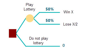
Now, you can ask yourself a question, if this X is 1000$, will you play the lottery, or won't play the lottery? (Remember the chance of losing 500$ in that case). If yes, then ask again, what about 2000$, or 10,000$ or more. The more the number you set as a winning number, half of that number can be a loss too. For example, if you set X = 50,000$, then 50% chance that you will win 50,000$ and 50% chance that you will lose 50,000$/2 = 25,000$. Are you willing to play such a lottery where you can lose 25,000$ in the hope of winning 50,000$? If so, that winning value of 50,000 is the value that you can use for R in your exponential utility function. If you think, you can afford to lose even more for the hope of gaining more, i.e., you can lose 100,000$ for the hope of gaining 200,000$. If so, then your Risk Tolerance value can be 200,000. In a word, think about the highest number that can be used for X so that you will be motivated to play the lottery.
Exact method (Certainty Equivalent Based)
Ok, we have demonstrated, how quickly we can approximate the value of the Risk Tolerance "R" by answering a question asked by the above decision tree. Now, let's see how we can get an Exact value of R mathematically. Consider a decision tree again, where, instead of answering the highest value of a winning payoff, you can answer the Certainty Equivalent of a given lottery. That means, say you can make a decision about playing a lottery with a 50% chance of winning the value of X and a 50% chance of losing a value Y. Or you can choose to receive a confirmed (Certain) amount of money, which can be very less than the possible highest outcome of the lottery. This certain amount of payoff is called "Certainty Equivalent".
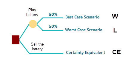
Anyway, let's consider the following decision tree. You have two options. One option is to play a lottery where you can Win "W" with a 50% probability, and you can lose "L" with a 50% probability. Another option is to receive a certain amount of money without playing the lottery. For example, Your friend is asking if you will like to sell that lottery for a certain amount of money. How much money you will ask for selling that lottery? Say, you asked "CE". Then, that CE is your certainty equivalent.
Now, let's see how we can use the concept of Certainty Equivalent to calculate an exact risk tolerance of an Exponential Utility Function.
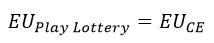
According to the theory of Expected Utility, and Von Neumann–Morgenstern utility theorem, if you can define a utility function, then your Expected Utility for the given gamble will be equal to your Certainty Equivalent. Because you will be indifferent between two options only if the Expected Utility of the tow options are the same. Here two options are either play the lottery or not to play the lottery for a certain amount of money.
The probabilities of winning and losing are both 0.5.
So, let's formulate the equation, where the EU stands for Expected Utility.
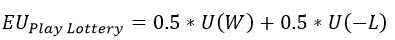
According to the theory of expected utility, the Expected utility of playing the lottery is equal to the expected utility of the Certainty Equivalent (CE).
Our Utility Function is the Exponential Utility Function which is 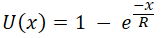
So, lets plugin this function to the above equation, after simplifying, we get,
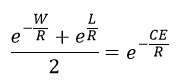
Here, W is the Winning amount from the lottery, L is the loss amount from the lottery, and CE is the certainty equivalent. All of these 3 values are constant. The only variable is R (Risk Tolerance). In order to find that value of R, the above equation needs to be solved. Solving such an equation is not very straight forward. It is a little complicated. But, when you have our Decision Analysis Software (Decision Tree Software or Rational Will), you won't have to worry about solving such an equation by yourself. Our software will solve that for you and tell you the exact value of "R". We will show you how to do that on this page, please keep continue reading.
Calculating Certainty Equivalent
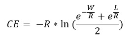
So far, we have developed an equation for finding Risk Tolerance. We can use the same equation to find the Certainty Equivalent of an Exponential Utility Function if all W, L, and R are known. In that case, it will be very easy to solve the equation. Because the left-hand side will just become a constant value. Just take the natural log of both sides and simplify as shown here.
Scaling Parameters
In real-life scenarios, you may want a utility function equation where the maximum payoff from an investment or lottery will yield the highest utility value (i.e. 1) and the minimum payoff (or loss) will give the lowest utility value. By introducing 2 parameters "a" and "b", the exponential utility function can be scaled such that,
That means, for different lottery or different scenarios, the value of "a" and "b" will be different.
How to find out the value of "a" and "b"?
Say, your highest utility is 1. For the given investment, your highest possible gain can be H and the lowest possible gain (or loss) can be L.
Then, your utility function with scaling parameters "a" and "b" can be mathematically derived as
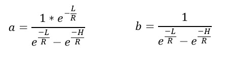
Say, in a lottery, you can gain a maximum of 1000$, and lose 500$. Then, setting these values, you can get "a" and "b" as
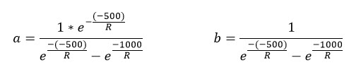
In the above equation, R is the Risk Tolerance, as usual. When you use the SpiceLogic Decision Analysis Software (Decision Tree Software or Rational Will), these scaling parameters will be evaluated automatically based on your other inputs.
Marginal Utility
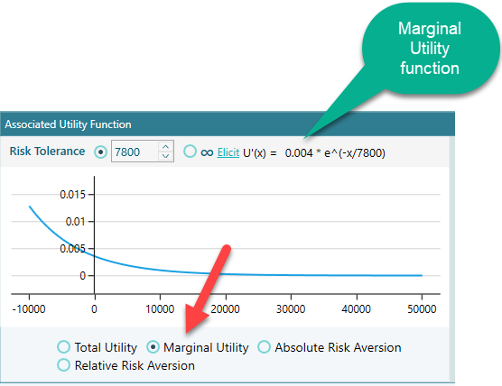
Marginal Utility is a measure that indicates how much a person's utility changes by a little change of payoff. Mathematically, if you differentiate the Utility Function U(x) with respect to the payoff x, then you get the Marginal Utility Function.
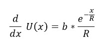
Here, the "b" is a scaling parameter, and R is the Risk Tolerance, x is the real-life payoff and U(x) is the utility value for the given payoff x.
Risk Aversions
Risk Aversion is a mathematical function that indicates how risk-averse a decision-maker is. The risk aversion function can be derived from the Utility function. As we explained in the Utility Function chapter that, the absolute risk aversion is

and the relative risk aversion is
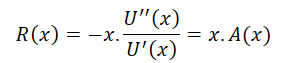
If we apply these operations on a scaled Utility Function equation, we get,


Notice that, the absolute risk aversion of an exponential utility function is a constant (1/R), that is irrespective of wealth. Therefore, the exponential utility function is most appropriate for people whose risk attitude does not change according to the amount of wealth they have. Many individuals might be less risk-averse if they had more wealth, which is the idea of the Bernoulli Utility Function.
Modeling Example
Say, you want to invest in a business where you hope to make a lifetime revenue of 1,000$. But, you also fear that your initial investment of 200$ can be lost with a 50/50 chance. You need to make a decision about that investment. Should you invest or not? You decided to use an Exponential Utility Function to map your monetary gain to a perceived satisfaction. Why? Does not that more money means more satisfaction? Maybe, but more money comes with more risks too. So, you may need to be satisfied as soon as you get a certain target revenue. That's why a utility function makes a big sense.
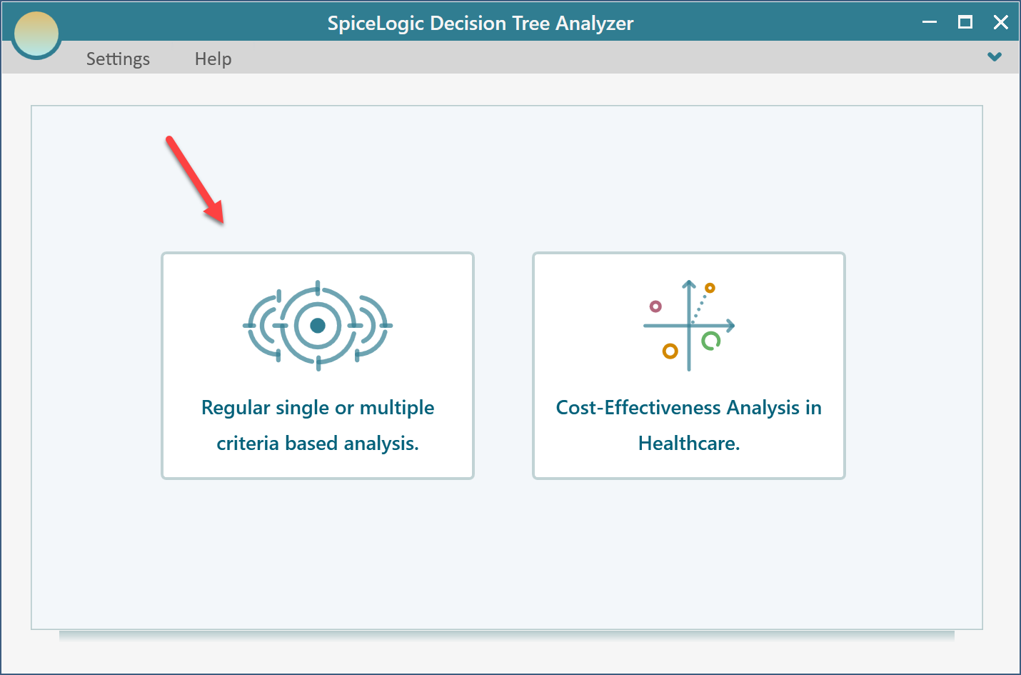
If you are using the SpiceLogic Decision Tree Analyzer software then you will be greeted with the following screen. If you are using Rational Will software, click the "Decision Tree" button from the home screen to get to this view. Click the button "Set up Criteria".

Once you click that button, you will be asked, if you want to use a regular single/multiple criteria analysis or Cost-Effectiveness analysis. Choose the first option.
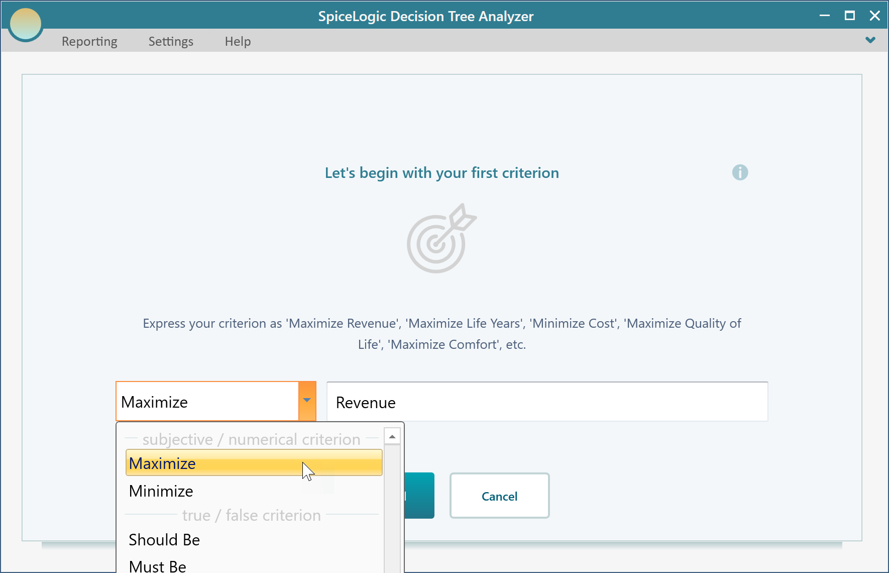
Then you will be presented with the following screen. Select "Maximize" and enter "Revenue" as shown below.
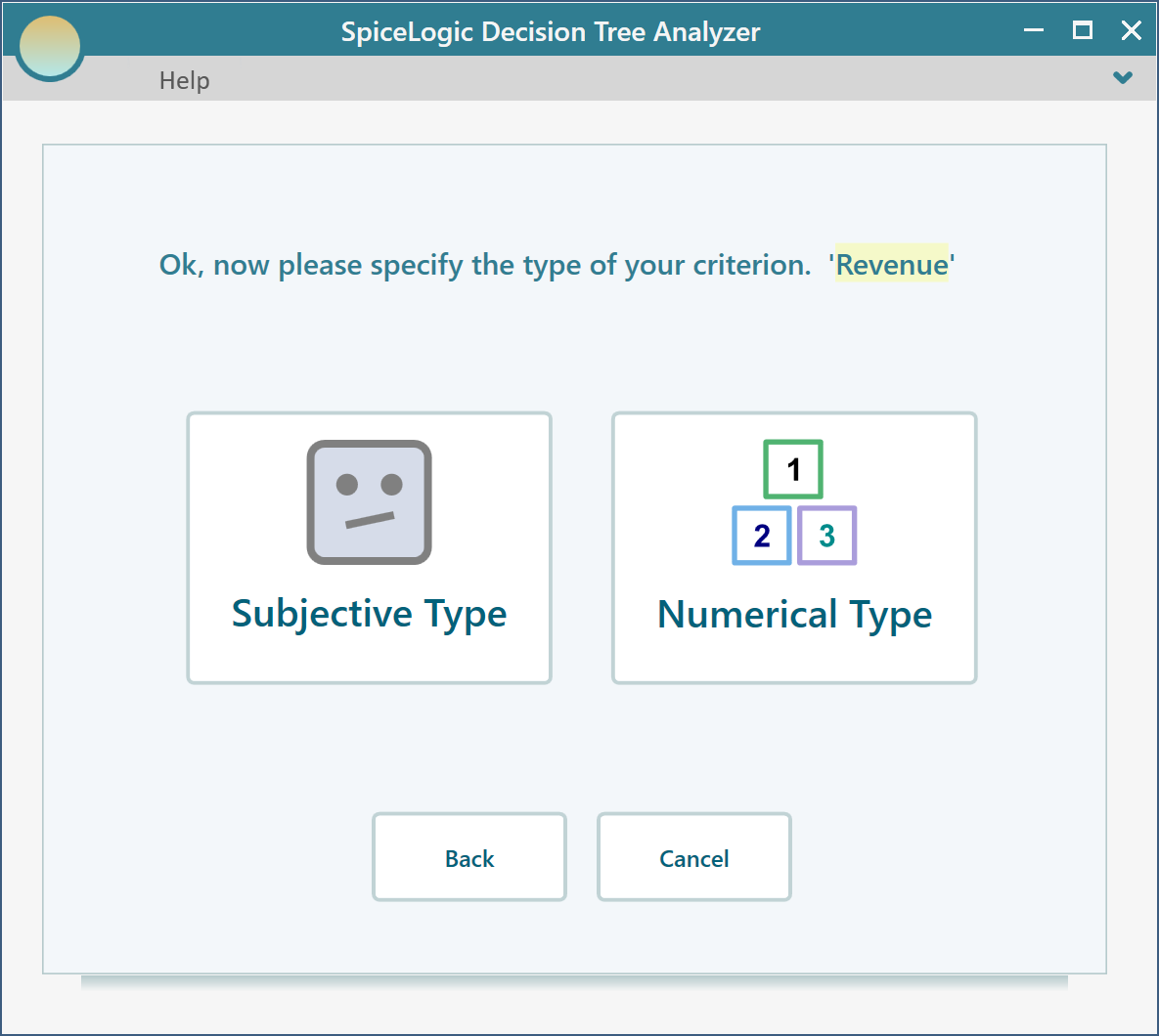
Then click the "Proceed" button. You will be asked about the type of criterion. Select "Numerical Type". Please remember that, in order to use a Utility function, you need to use the Numerical type criterion.
Then you will be asked about the minimum, maximum payoff range from the investment. Enter Minimum = -200 (as you may lose an investment of 200$) and maximum = 1000.
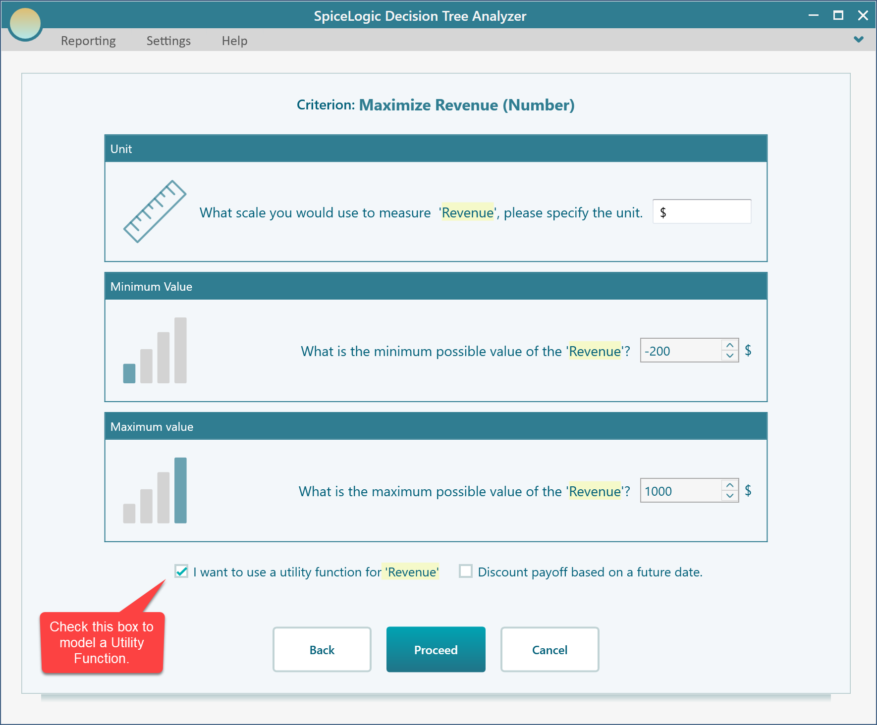
Click Proceed. As you have checked the box "I want to use a utility function...", you will be presented with a utility function editor. Select the "Exponential Utility Function" button.
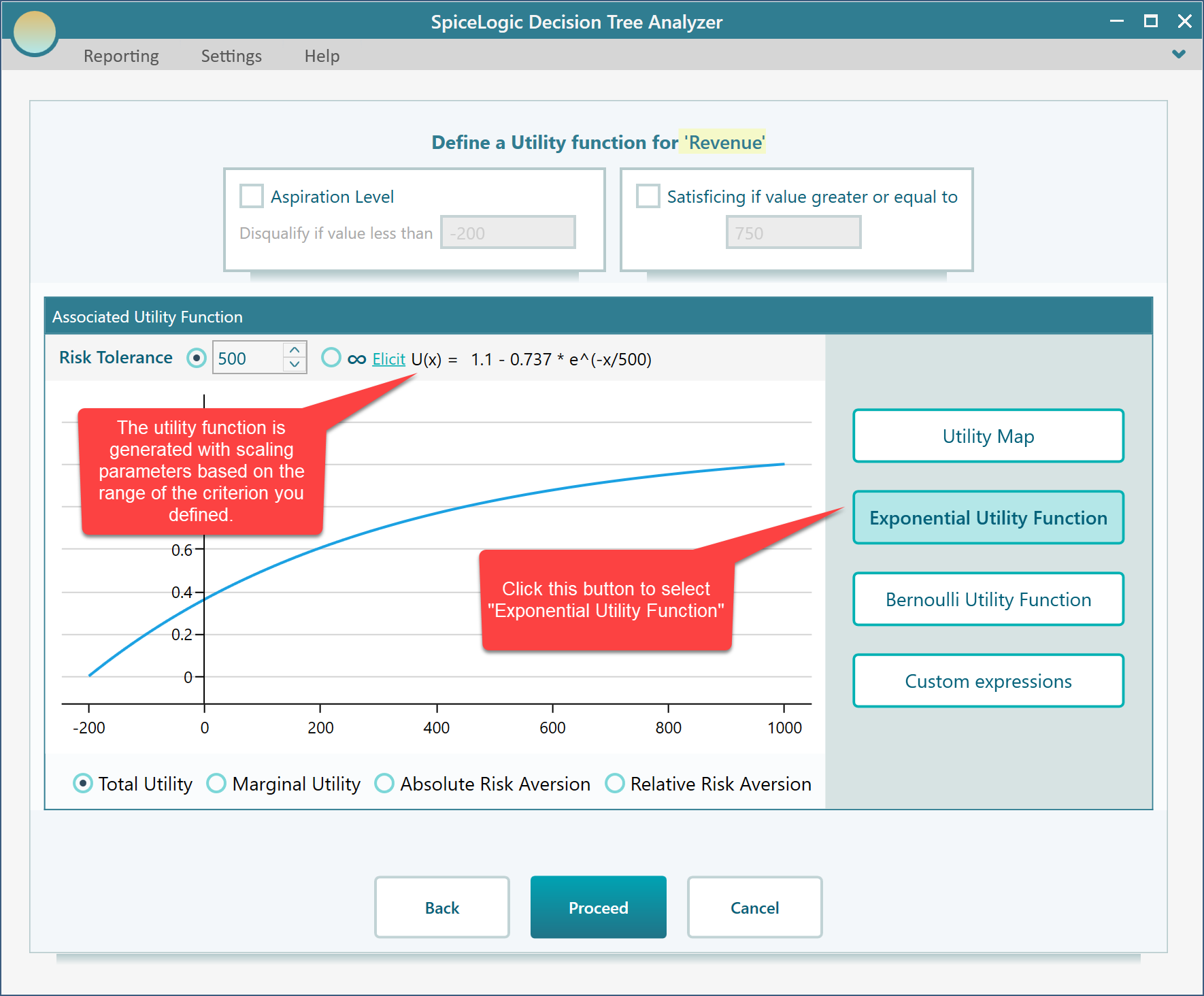
In the above screenshot, you can see that an exponential utility function is automatically evaluated for you with calculated scaling parameters.
How Scaling parameters are calculated
You may be curious to know, in the generated utility function, from where these scaling parameters 109.98 and -73.72 come from. The scaling parameters are calculated such that, the maximum payoff will result in the highest utility value which can be 1 or 100, depending on the preference. The lowest payoff will result in the lowest utility value which can be 0, or -1, or -100, depending on the preferences. The preference can be specified from the ribbon as shown here.
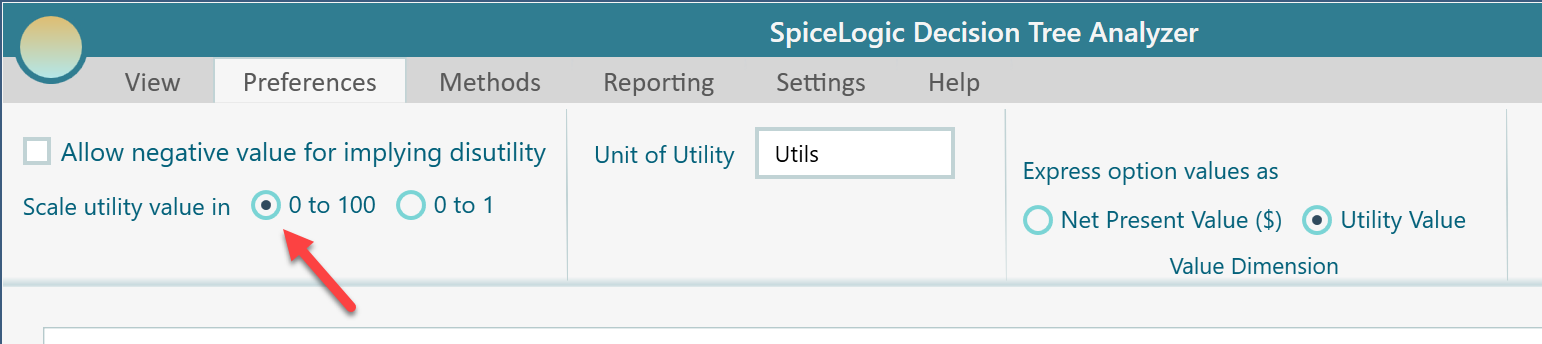
Let's set the utility value scale as 0 to 100. It is up to you but the following examples are used based on 0 to 100 range.
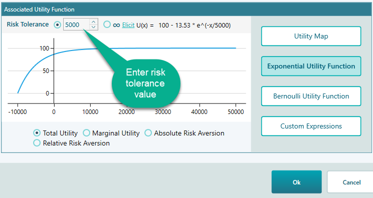
Specifying Risk Tolerance
The most important parameter in the Exponential Utility function is 'Risk Tolerance'. You can directly enter the Risk Tolerance value here, as shown in the following screenshot.
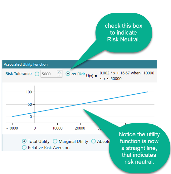
If you are completely risk-neutral, your Risk Tolerance value should be infinity. You can set that by clicking this radio button.
Eliciting Risk Tolerance
As we have explained, there are two ways to elicit the Risk Tolerance value (R) of an exponential utility function. Approximate method and exact method. An approximate method is easy to understand and use but as you have our software at hand, why don't you start with the Exact method as all complicated calculations are done by the software.
Exact method
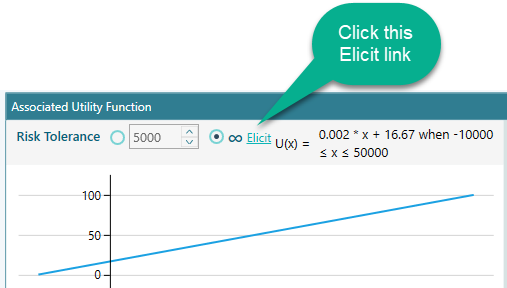
In order to use the Exact method to elicit your Risk Tolerance, click the "Elicit" link as shown below.
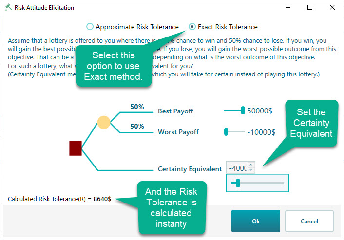
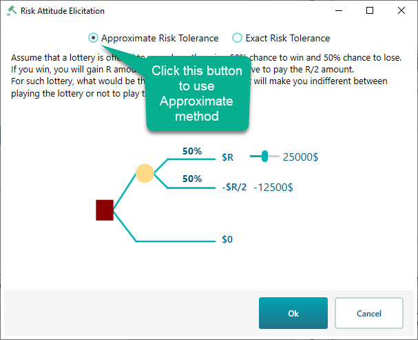
Once you click that link, you will see the following window. Where the "Exact Risk Tolerance" method is checked by default. You will see that a decision tree is already populated with the Best Payoff = Maximum value of the criterion and Worst Payoff = Minimum Value of the criterion, which was entered by you previously. Of course, you can change those numbers using the given sliders. Once you completed setting up the Best Payoff and Worst Payoff, Enter a Certainty Equivalent value using the slider as shown here. You will see a risk tolerance value is calculated instantly.
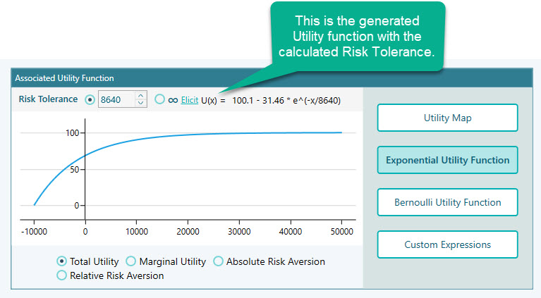
If you click OK, you will see the calculated risk tolerance is passed to the Exponential Utility function editor.
Approximate method
You can also check how the approximate method can be helpful to find your Risk Tolerance "R". Click the radio button "Approximate Risk Tolerance" as you can see in the following screenshot. There, you will see a decision tree where the Winning amount is set as the maximum value of the criterion entered by you. The losing amount is auto-calculated as half of the winning amount. Using the slider, think about the highest number for what, you are willing to play the lottery given that, half of that winning amount can be lost by 50% chance as well.
Viewing other derivatives of the generated utility function.
Not only the generated exponential utility function, but you can also see various derivatives of the utility function from the Decision Analysis software (Decision Tree Software, or Rational Will). You will find a set of radio buttons at the bottom of the chart as shown in the following screenshot. Say, you click the radio button for "Marginal Utility", you will see the generated Marginal Utility Function equation, along with a plot as shown here.
You can find a similar view for Absolute Risk Aversion and Relative Risk Aversion as well.
Finally, model the Decision Tree
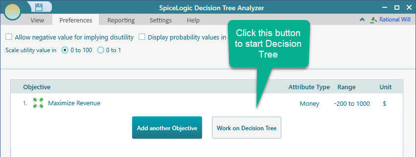
Click Ok in your Objective editor when you are done refining your utility function. Then, you will be taken to the Objectives manager page. Click the "Work on Decision Tree" button.
Then, click the "Decision Node" button to create your decision tree that starts with a decision node.

Then, create a decision tree like this. If you are not familiar with how to create the decision tree in our decision tree software, please visit the getting started page. From that page, you will know how to set a payoff to a node.
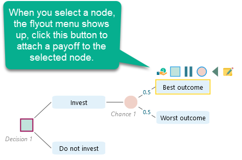
Set payoff 1000$ for the Best outcome, -200$ for the Worst outcome, and set 0 for the 'Do not invest' node.
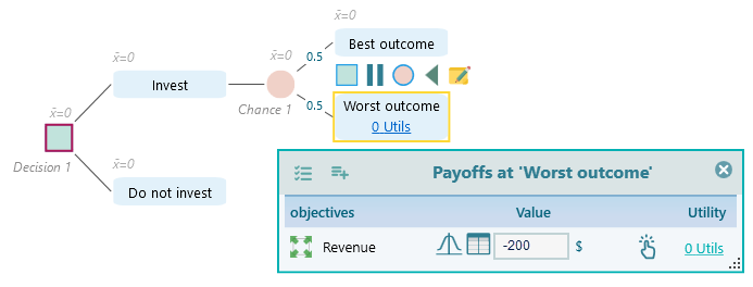
Finally, when all node payoffs are set, the decision tree will look like this.
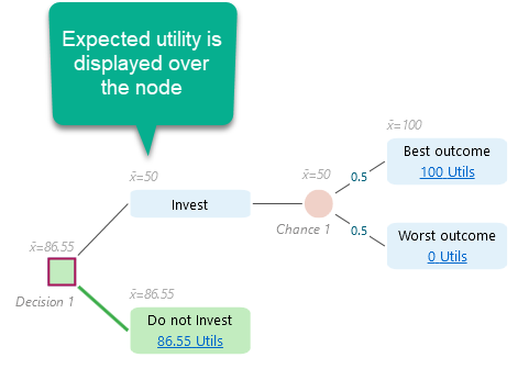
Note that, the numbers in utils shown on the Decision Tree nodes, are actually calculated utility values. You need to enter the real payoff and then the utility values are calculated based on the utility function. For example, the node "Do not Invest" is showing 86.55 Utils. Why? Because, the exponential utility function we modeled, the utility value for 0 is 86.55. As the real payoff for "do not invest" is 0, the above utility is calculated and shown. For the Worst outcome node, we entered the value = -200, which was evaluated as 0 utility. And we entered the payoff value for the Best Outcome node as 1000, which was evaluated as 100 Utils according to the generated exponential utility function.
Also, notice that the Expected Utility is calculated and shown over the node. As you can see, the expected utility for the "Invest" node is shown as 50 Utils, which is less than the option "Do not invest", therefore, the Node "Do not Invest" is shown highlighted with green color, indicating the recommended strategy.
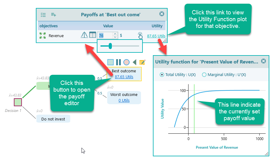
Click the Utils link on any node, you will see the payoff editor opens up. From there, you can see the payoff and the utility function plot. In that plot, you can also see a green vertical line that indicates where your utility stands in the plot based on the currently set payoff. The line moves as you change the payoff instantly.
Finally, we hope, you enjoy the Decision Analysis software (Decision Tree Analyzer or Rational WIll) while modeling your exponential utility function.