Modeling Markov Chain and Markov Decision Process
SpiceLogic Decision Tree Software lets you model a Markov Chain or Markov Decision Process using a special node called Markov Chance Node. You can set reward (or Payoff) to a Markov State or Markov Action and perform Utility Analysis or Cost-Effectiveness Analysis for that Markov Chain or Markov Decision Process.
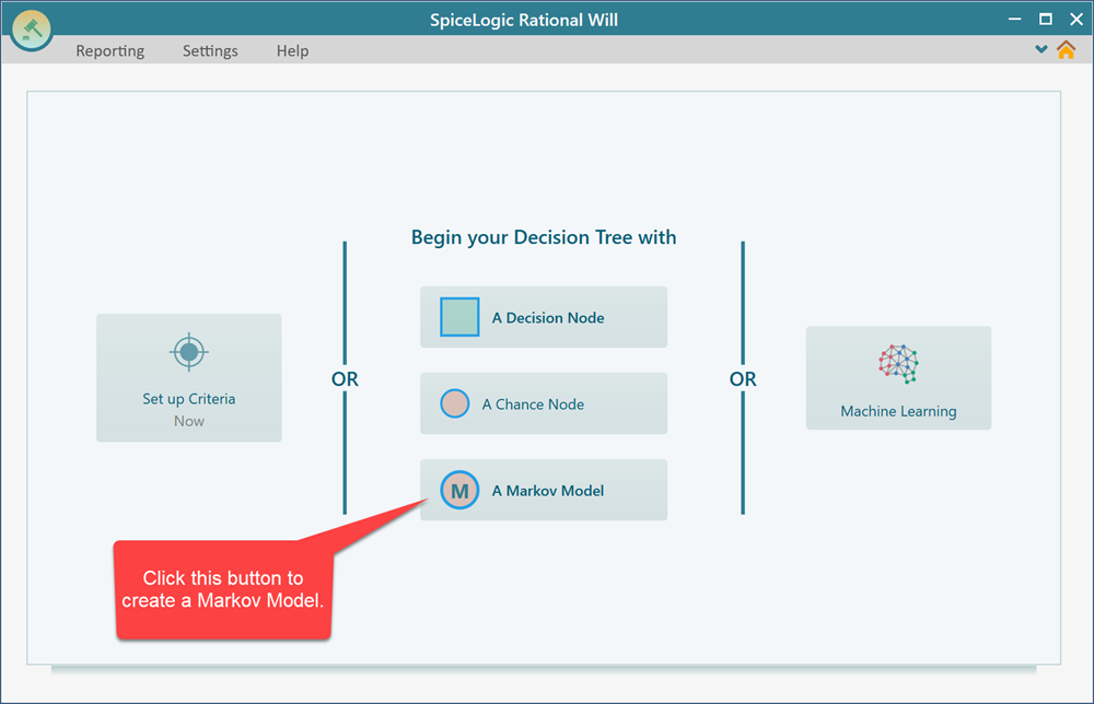
Same as Decision Node or a Chance Node, you can use a Markov Chance Node as a Root node as you can see that option in the software start screen. When you start the Decision Tree software, you will see the button "A Markov Model". Click that button and you will get a decision tree where the root node is a Markov Chance Node. But, before getting to the Decision Tree diagram view, you will see a Step by Step wizard show up so that you can easily answer questions about what will be the Markov States, their transition probabilities, etc. Then a Markov diagram will be created for you.
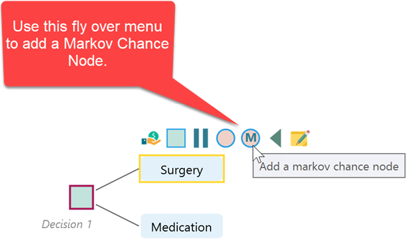
If you have already created a decision tree, you can attach a Markov model to an action node as shown in the following screenshot.
Wizard for creating the Markov Model
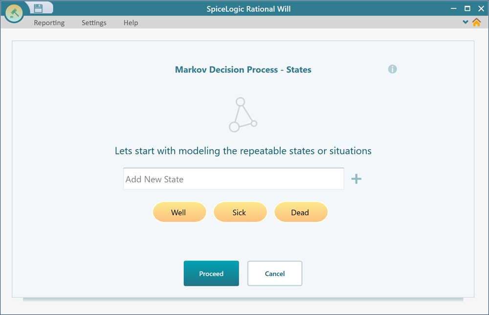
Once you click the Markov Chance node button or the Markov Model button, you will be presented with a Wizard for creating your Markov model step by step. A Markov Chain or a Markov Decision Process is built with the Markov States. Markov State is similar to a Decision Tree Chance node, but unlike a Decision tree chance node, a Markov state can be cyclic. That means a State can transition to another state and come back to the same state. You can add as many states as you want from this interface and proceed.
In the wizard, you will be asked about setting transition probabilities, creating actions, configuring criteria or cost-effectiveness parameters, and finally setting utility values or cost/effectiveness values for a state or an action. Here is a screenshot of a step where you can specify the transition probabilities of a state.
![]()
Following the Wizard is really a straightforward process. Just try out and you will not get lost. Once you finish the wizard, a Markov model will be created and you will see a decision tree-like diagram for your model. You are not forced to use the wizard for creating the model. You can simply click the Cancel button and then you will be taken to the diagram where you can manually add states, set transition probabilities, etc. In the following section, you will learn how to modify your Markov Model which is already created by the wizard. Also, the same knowledge will apply if you choose not to use the wizard, rather you want to do everything manually.
Creating Markov State from the diagram
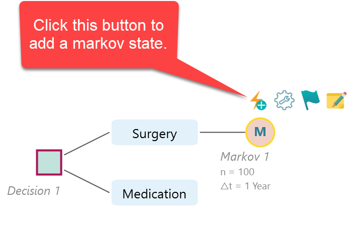
Once you add a Markov Chance node, same as a regular decision tree chance node, you can add states as children of the Markov Chance node.
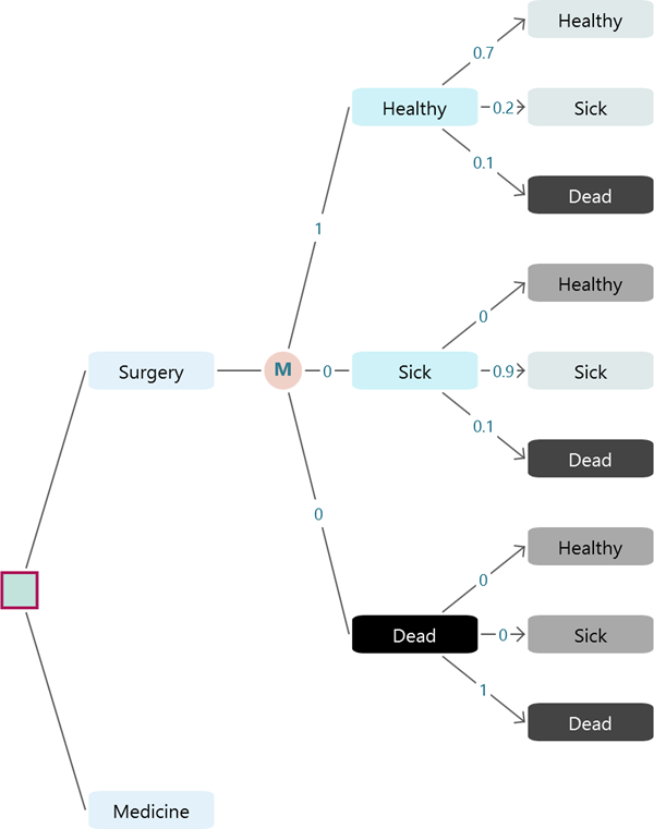
Say you added three states under a Markov Chance node and named them "Healthy", "Sick", and "Dead", you will see that all the state nodes are connected to each other in order to complete a Markov transition system.
Accessing Markov Settings from the diagram
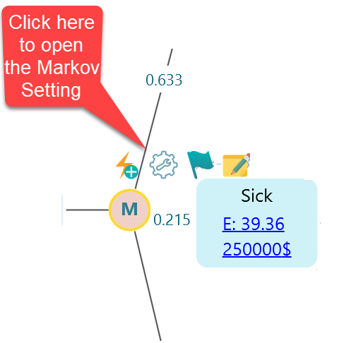
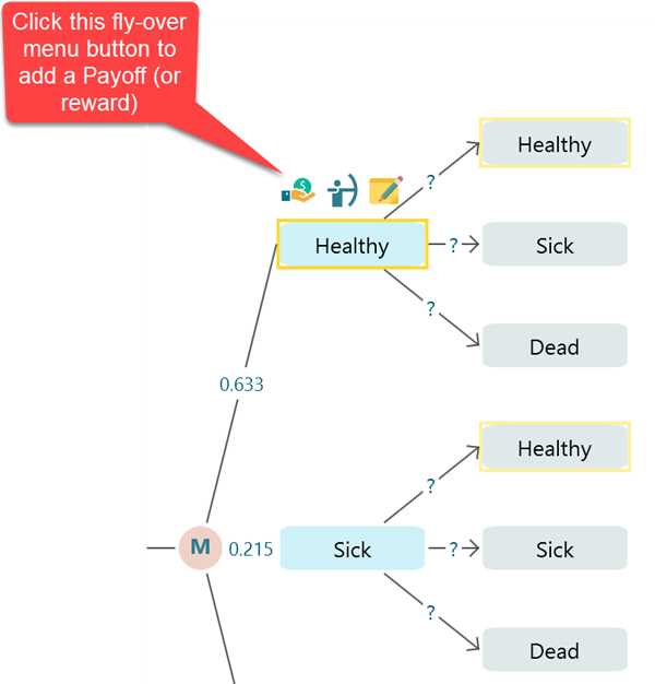
Probably it is better to review and set up your Markov Simulation setting before performing the simulation and setting up transition probabilities. The decision tree software will execute a cohort simulation to solve the Markov Chain or Markov Decision Process. You can define the cohort simulation setting by clicking this fly-over menu icon from the Markov Chance node.
Once you click that button, the Markov Cohort Simulation setting for that chance node will open up as shown below.
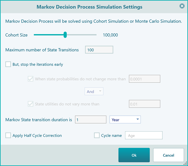
Cohort Size: Notice that there are several things that you can set here to customize your Experience with the Simulation result. The first thing is the Cohort Size. By default, the software uses 100,000 which is really good enough for any scenario, and therefore you may not need to change this setting. But feel free to change it if you want and see how the result gets a little better for a big number.
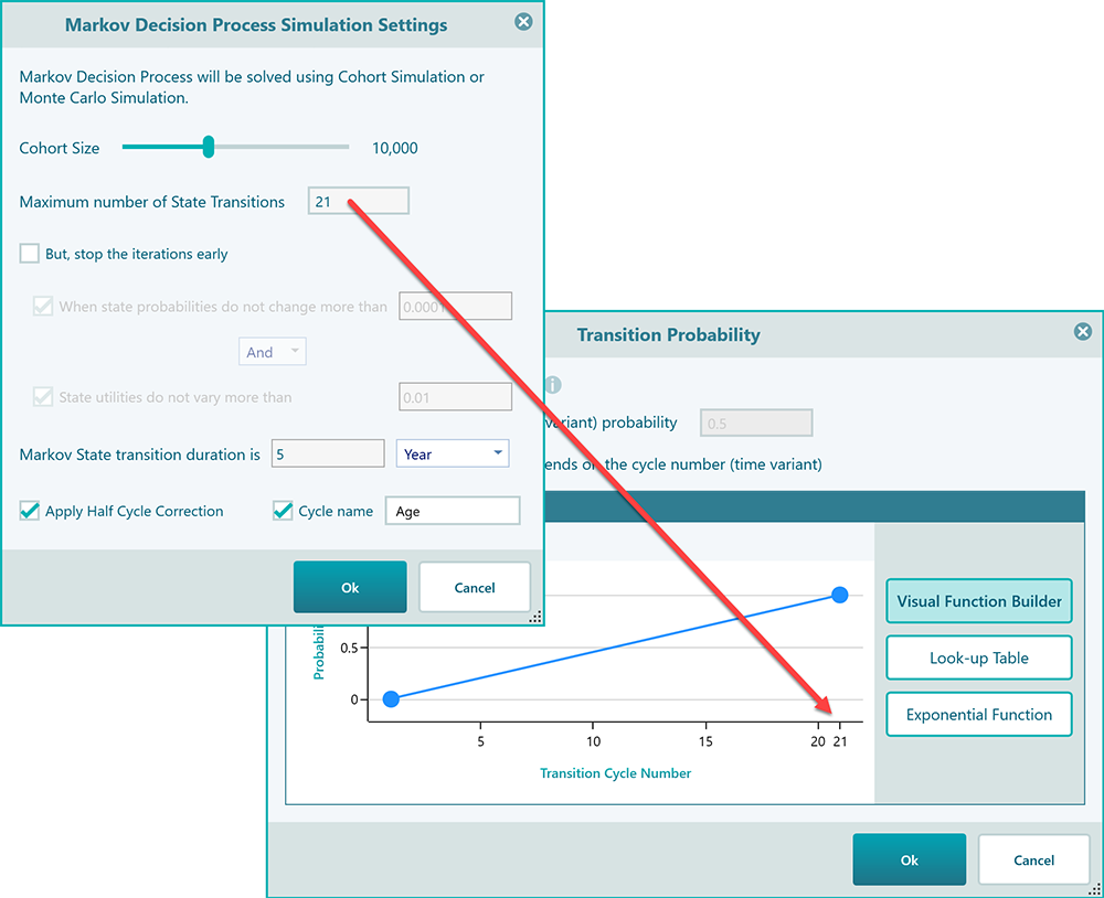
The maximum number of state transitions: The next setting is the maximum number of state transitions. The software uses 100 as default, which is fair enough for any regular Markov simulation but for healthcare applications, you may need to set that based on exactly how many years of prediction you want. For example, you may want to analyze a treatment effect for the next 10 years, so, set that number 10 in that case.
Convergence setting: After that, you will find a convergence setting. That means you can tell the program to stop transitions early if the probabilities of a state do not change or converge. You can set up if the probability change should be tracked to stop or state utility value should be tracked to stop early. You can choose both, either / or/and combination as you can see from the above screenshot.
State Transition duration: Then, you will see the state transition duration setting. This setting is especially useful for calculating a discounted value for a future time. Say, your Markov cycles are 5 years apart, the utility values that every cycle gets will be discounted based on that future date. Not only that, if your transition probabilities are based on the fact that every transition cycle is 5 years apart, then you will have to set the state transition duration accordingly to make the probabilities correctly applied. The value you choose here for state transition duration will be reflected in the charts, tables, and reports.
Half-cycle correction: You see a checkbox "Apply half-cycle correction". It is a straightforward thing. Usually, in healthcare analysis, we apply half-cycle correction especially if the Markov state transition is a long time. So, apply half-cycle correction by checking this box. If you are not sure what to choose, then leave it unchecked as in the most regular models, this is not required.
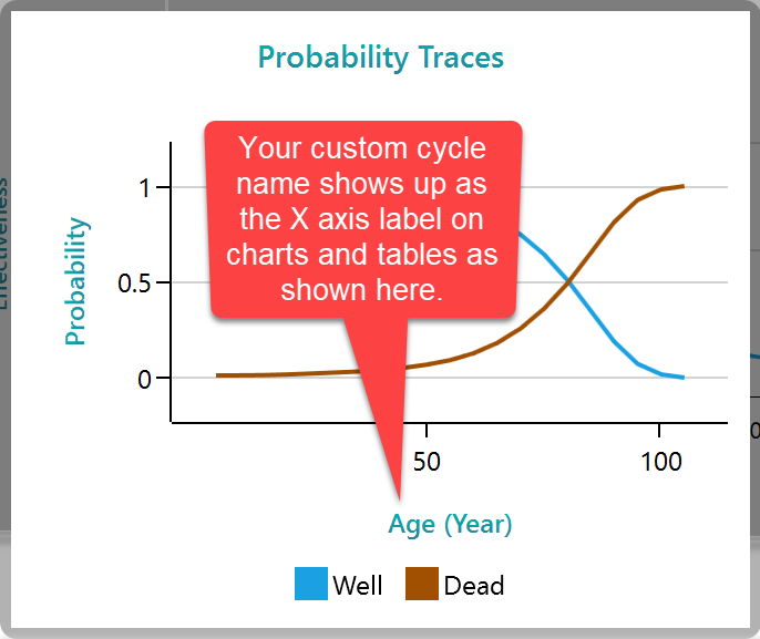
Custom cycle name: The last setting is using a custom Cycle name. If you are analyzing the life expectancy of a cohort, then obviously your probability transitions will be based on the age of the cohort, right? Instead of seeing the cycle number in the charts and tables, it will be useful to see the "Age" as the X-axis label, right? So, if you want to give the name of the transition cycles for a better reporting experience, check this box and give a name to your cycle number. By default, the program shows the name "Age" which is common for most healthcare analyses. Here is a screenshot that shows how this custom cycle name is applied so that you can get an idea about why you may like to use a custom label for your cycle number.
Setting Initial Probabilities from the diagram
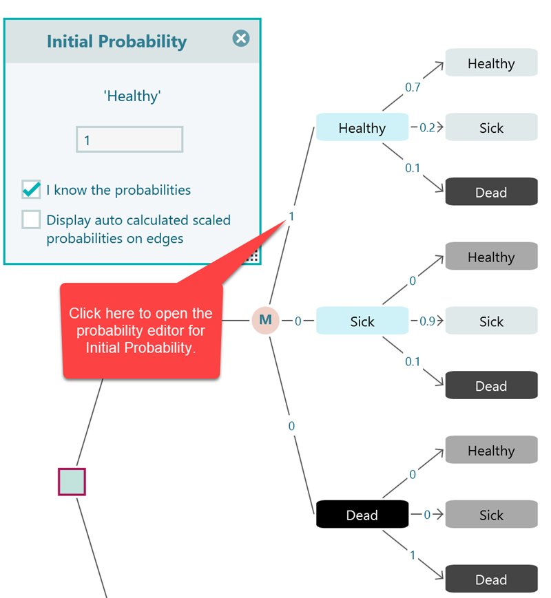
In a Markov chain or a Markov decision process, you need to specify the initial probabilities of the states in the system. For example, there can be three states "Healthy", "Sick" and "Dead". You may define that the population has a 20% chance to start as well, a 50% chance to start as Sick, and a 30% chance to start as Dead. These are called initial probabilities. But, practically, you may find that the population always starts from one given initial state. So the initial probability for that state will be 1 and the rest of the state's initial probability will be 0.
In order to set the initial probability of a state, you can click on the probability number or the '?' shown on the edge as shown here.
Setting Initial State from the diagram
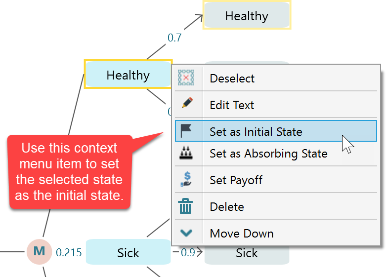
There is a shortcut way to set a state as an Initial State. Just select the Markov State and right-mouse click to bring the context menu. You will find a context menu option for setting the selected state as the initial state. If you choose this option, then the initial probability of that selected state will be set as 1 and the rest of the state's initial probability will be set as 0.
Setting Transition Probabilities from the diagram
In a Markov Chain or a Markov Decision Process, you need to connect the states with transition probabilities. You can easily set the transition probabilities almost similar to how you set a probability of a regular chance node event. Once you see the Markov system is completed like a tree as shown below, click the highlighted numbers or '?' for setting the transition probabilities.
![]()
Once you click there you will see a transition probability editor shows up like this.
![]()
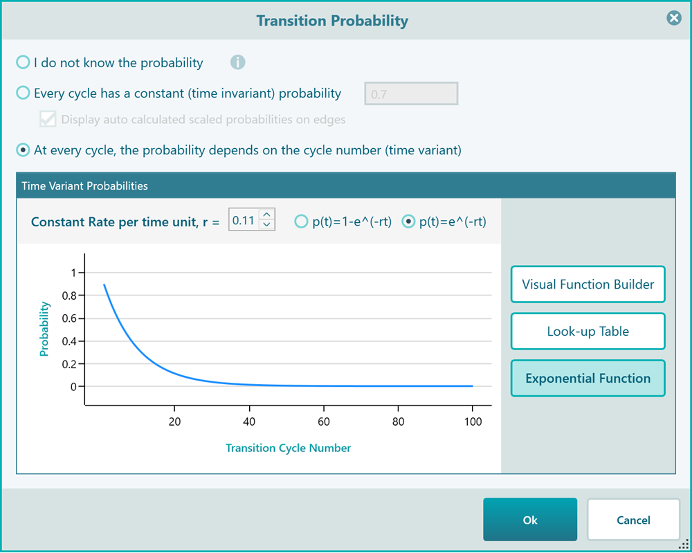
Time variant probabilities
SpiceLogic Decision Tree software lets you define a probability function so that you can have different probabilities based on the cycle number in the cohort simulation. That option is especially useful for modeling healthcare situations where a cohort will have different probabilities of getting sick when age increases. In real life, a patient's probability to get a stroke or die increases as the patient get more ages, right? So, you cannot use a constant probability for such a transition. If you check the last box to use a time-variant probability, you will see a lot of options for using a time-variant probability.
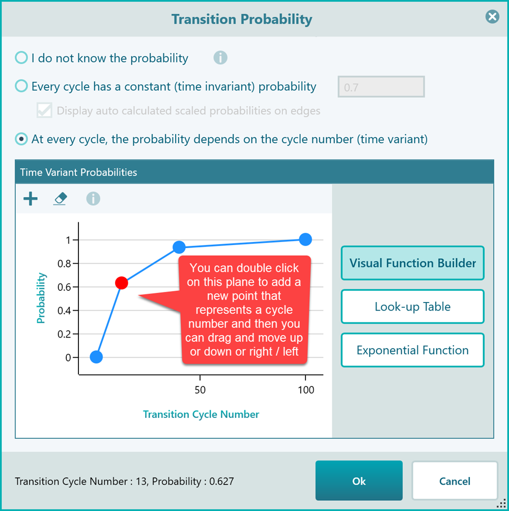
As you can see, this visual function builder is a very intuitive way to create a time-variant probability function. Just double click to add a new point, and use your mouse to drag and move up/down or right/left. You can select a point and hit the DELETE key to delete the point. The next option is using a Look-up table as you see in the following screenshot.
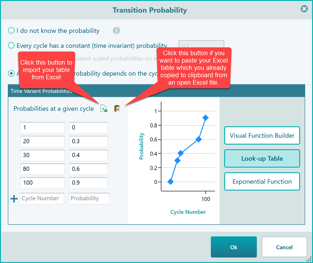
You do not need to fill the table with all cycle numbers. The software will interpolate the probability value based on the given cycle number entries in the table.
Finally, you can use an Exponential Function if you have a constant rate, as shown below.
You may wonder, why the charts and table inputs show the X-axis numbers up to 100. Actually, this 100 is coming from your Markov Settings where you have specified the maximum number of state transitions. Say you change that to 21, then in the time-variant probability panel, you will see all charts and tables showing max X value 21.
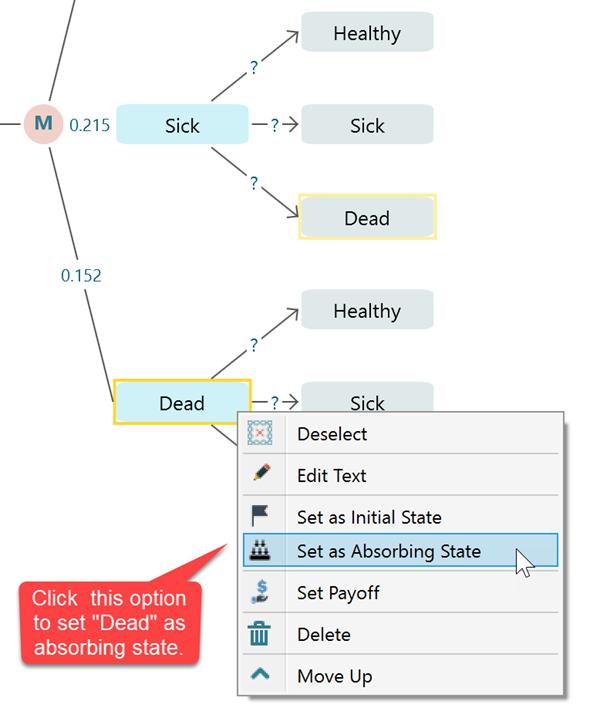
Setting a state as Absorbing State
An absorbing state is a state where, once entered, cant be left. A very practical example of an absorbing state is a "Dead" state. When someone is Dead, he cannot transition to "Healthy" or "Sick". So, the transition probabilities of an absorbing state are such that, the transition probability from that state to itself will be 1 and the transition probability from that state to other states will be 0. If you set transition probabilities in that way, you will see the software will show that state in black color indicating that it is an absorbing state. In this software, there is a quick way to set a state as an absorbing state. Same as setting a state as an initial state, you can select the state and right-mouse click to bring the context menu. Then you will see the option "Set as absorbing state".
Adding action to model as a Markov Decision Process
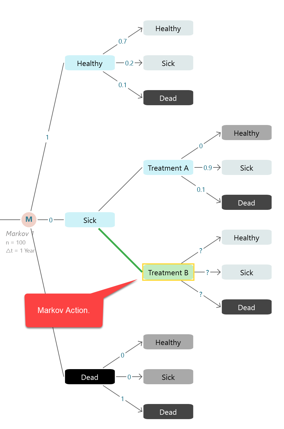
In a Markov Decision Process, you may have a few actions that can be taken from a given Markov state. For example, in the same given Markov chain, you may think that, if the patient gets sick, you can perform two actions, "Treatment A" and "Treatment B". You want to know which action will give the best quality-adjusted life year. Yes, you can find a policy for that.
You can add one or more Markov Action nodes as children of a Markov State node.
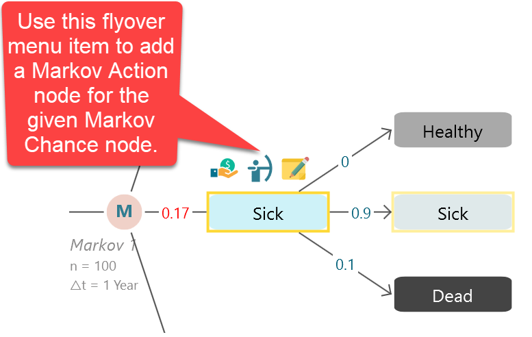
Say, you want to define two actions as Treatment A and Treatment B for the state Sick. You can use that button to create them,
You will find that the evaluated policy will be shown in the Markov Analyzer panel.
Setting Reward (or Payoff)
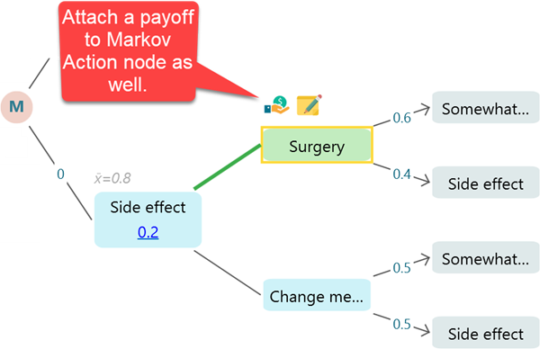
Same as a regular payoff to a Decision Tree action or event node, you can add a Payoff or Reward to a Markov State or a Markov Action node. You can use a Cost-Effectiveness analysis on a Markov Chain that is very common in healthcare.
Here is an example of using QALY and Cost as Payoff. You can use DALY or regular effectiveness variable as well.
.png)
Analyzing Result Charts and Tables
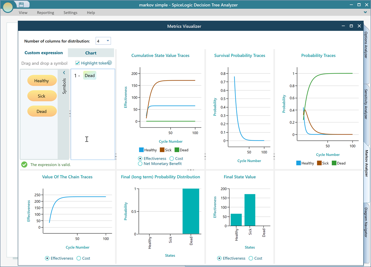
Ok, once you have completed the model, you will find a lot of useful metrics, charts, and tables are calculated and displayed in the Markov Analyzer tab. Expand the Markov Analyzer tab as shown below and you will see a result like this. Notice that, you can export the table to Excel for further analysis easily by an obvious Excel button.
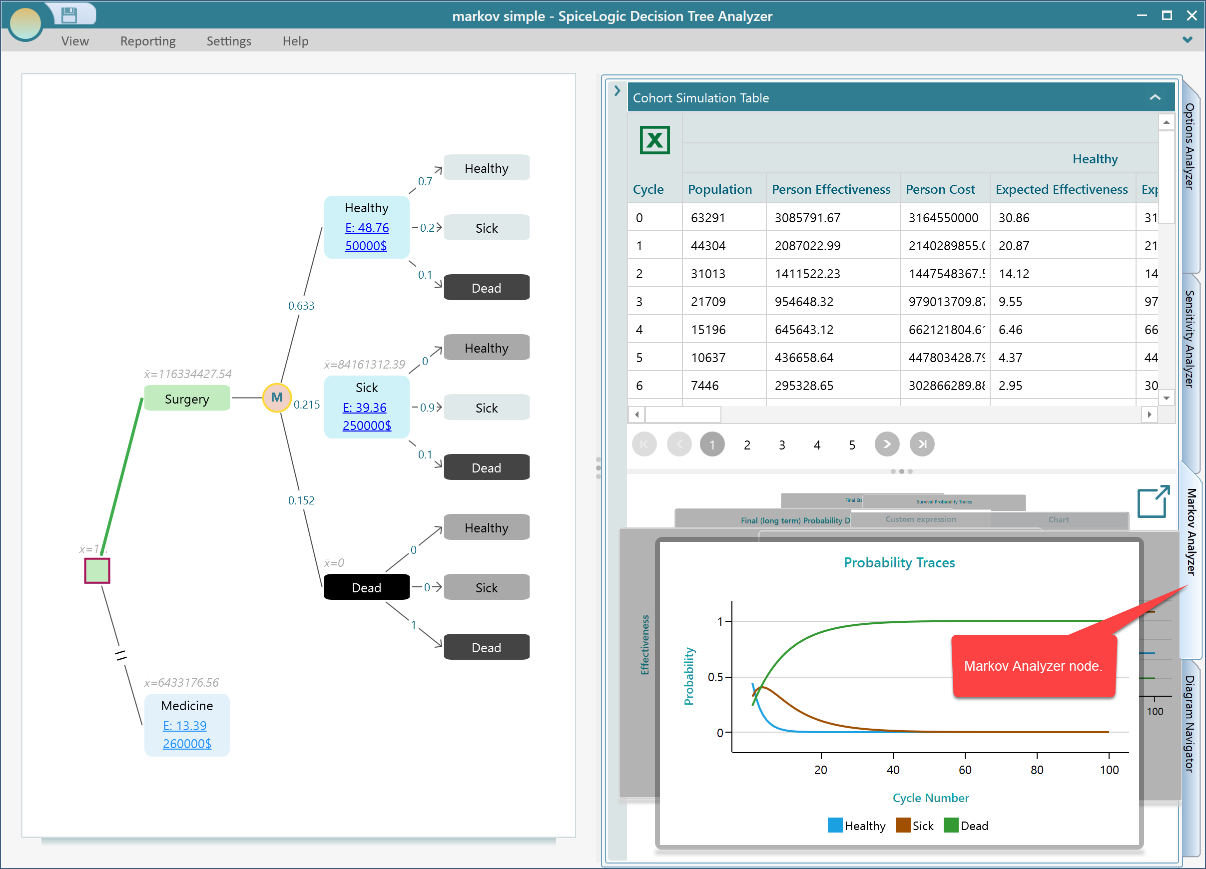
You can click that Pop-out button to see all the charts in a separate window instead of a carousel.
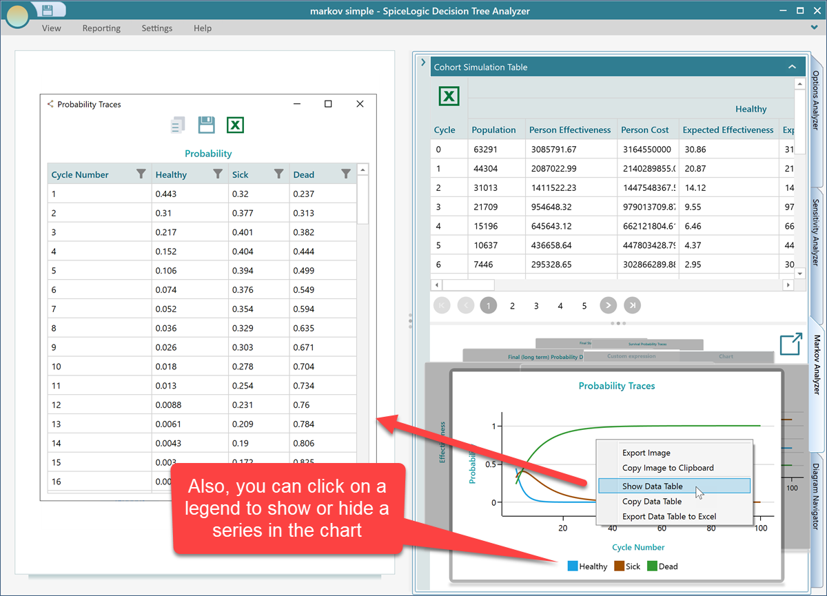
As you might know, in this software, every chart is featured with some common data export feature. You can right-click on a chart to see its context menu. You will find options for showing the data table that is used in the chart, exporting the table to excel, copying the image into clipboard or exporting as an image, etc.
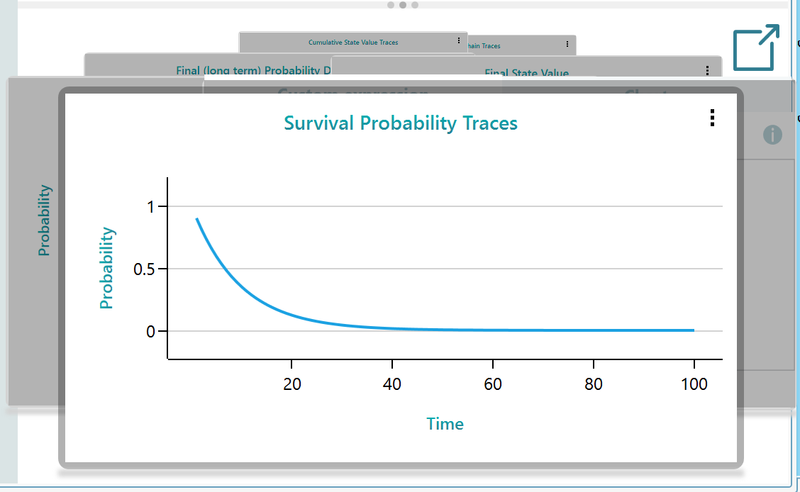
Survival probability
Notice that, there is a dedicated chart showing Survival probability. Yes, when there is a state defined as an Absorbing state, the software understands that the survival probability is the probability of living in any other state except an absorbing state.
Custom State Expression
You can have curiosity like "What would be the probability of STATE A and STATE B BUT NOT STATE C...
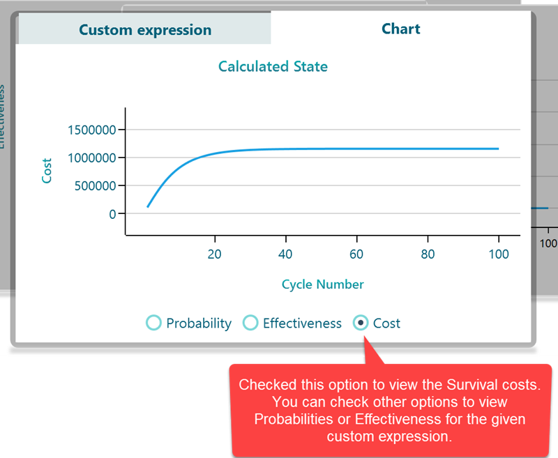
Yes, this software supports Custom Expression for querying sich expression, and then it will display a chart based on that query. Just select the Custom Expression in the carousel. Even though we have a dedicated chart for displaying Survival Probability, say, there was not any survival probability chart. You want to model a custom expression to find out the survival probability over cycles.
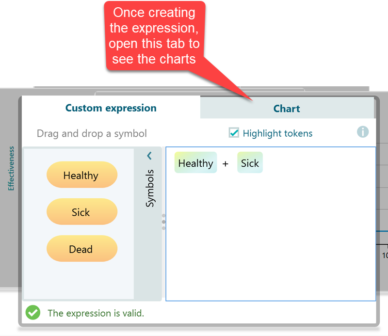
Once you open the Chart tab, you will see you have the option to view charts for Probability traces, Costs, or Effectiveness for living in these states.
Discounting Markov Cycle Payoff
If you set an interest rate that can be used to discount a future payoff, then all of your future Markov Cycle payoff will be discounted based on that interest rate. For example, in the Cost-Effectiveness Criterion editor, there is a section at the bottom to set up interest rates for discounting.
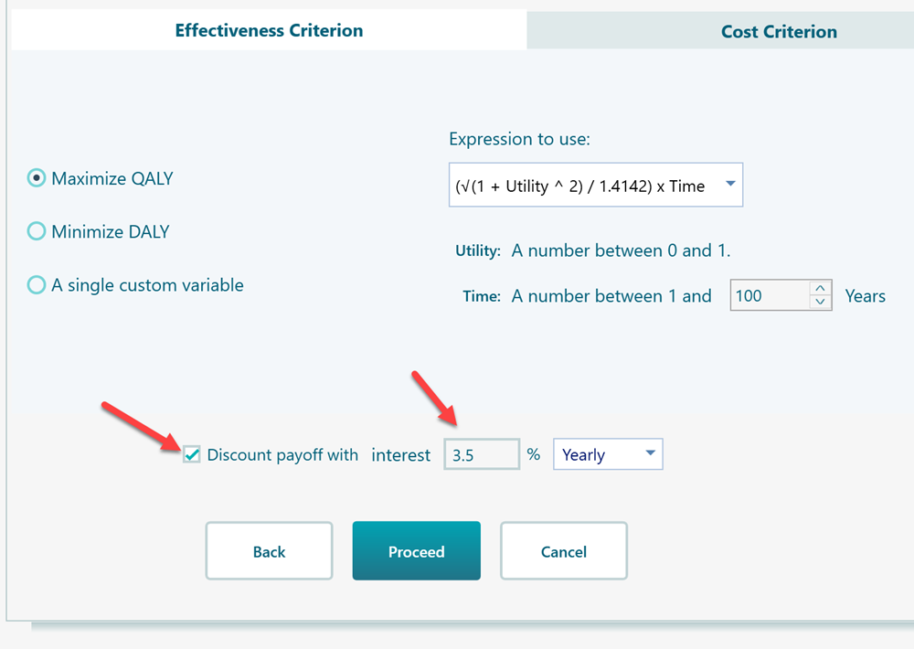
If you set that box with an interest rate > 0, then, your Markov cycle number will be considered a future event. The event year will be calculated based on the Markov cycle duration. And then, the payoff of that cycle will be discounted accordingly.
Conclusion
I hope, you found this article useful. Please try the features by yourself and you will discover a lot of more effective ways to use this software.