Example: Modeling Base Rate Fallacy

The base rate fallacy is also known as base rate neglect or base rate bias.

When evaluating the probability of an event―for instance, diagnosing a disease, there are two types of information that may be available.

1. Generic information about how frequently an event occurs naturally. Suppose, according to the statistics, 1% of women have breast cancer. So, this information is general information.
2. Specific information about an event in a given context. For example, 80% of mammograms detect breast cancer when a woman really has breast cancer.

When presented with both types of information at the same time, type 1 information is called "base rate" information.

When we have just the generic information, it is okay to assume the probability of an event based on that generic information. But when we have more specific information, our brain tends to judge the probability of an event based on that specific information and neglect the base rate information. That's why it is called base rate neglect too. (neglecting the base rate). Neglecting the base rate information in this way is called Base Rate Fallacy.

Using Rational Will or the Bayesian Network Software from SpiceLogic, you can incorporate these 2 types of information to judge a probability of an event or a hypothesis.

Real-Life Example

Let's apply that concept in a real-world example. Suppose, we have generic information, "1% of women have breast cancer". Also, we have specific information - "80% of mammograms detect breast cancer when a woman really has breast cancer". Another specific information we collected was that "9.6% of mammograms detect breast cancer when it's not there (false positive)".

Now suppose a woman gets a positive test result. What are the chances that she has cancer?

[Calculation]

Let's define some variables.
C = "Cancer".
R = "Positive Test Result"

As 1% of women have breast cancer. Probability of Cancer in general = Pr(C) = 0.01. This is what we call base rate.
Pr(R|C) = Probability of the positive test result (X) given that the woman has cancer (C). This is the probability of a true positive. According to our information,
Pr(R|C) = 0.8.
Pr(not C) = Probability of not having cancer = 1 - 0.01 = 0.99
Pr(R|not C) = Probability of a positive test result (R) given that the woman does not have cancer. (~C). This is the false positive. = 9.6% = 0.096

Now, we need to find out Pr(C|R) = the probability of having cancer (C) given a positive test result (R).

According to Baye's theorem,

Pr(C|R) = Probability of the woman has cancer given the positive test result
= Pr(R|C) * Pr(C) / (Pr(R|C) * Pr(C) + Pr(R|not C) * Pr(not C))
= 0.8 * 0.01 / ( 0.8 * 0.01 + 0.096 * 0.99)
= 0.0776
= 7.76%. 

You can model this problem in the Bayesian Network Software or the Rational Will and get the same result easily without doing the calculation by hand. The software will give you a pleasing way to visually depict the problem and see the result in the graphical interface.

Modeling base rate fallacy in Bayesian Inference

Start the software and choose the "Bayesian Inference"

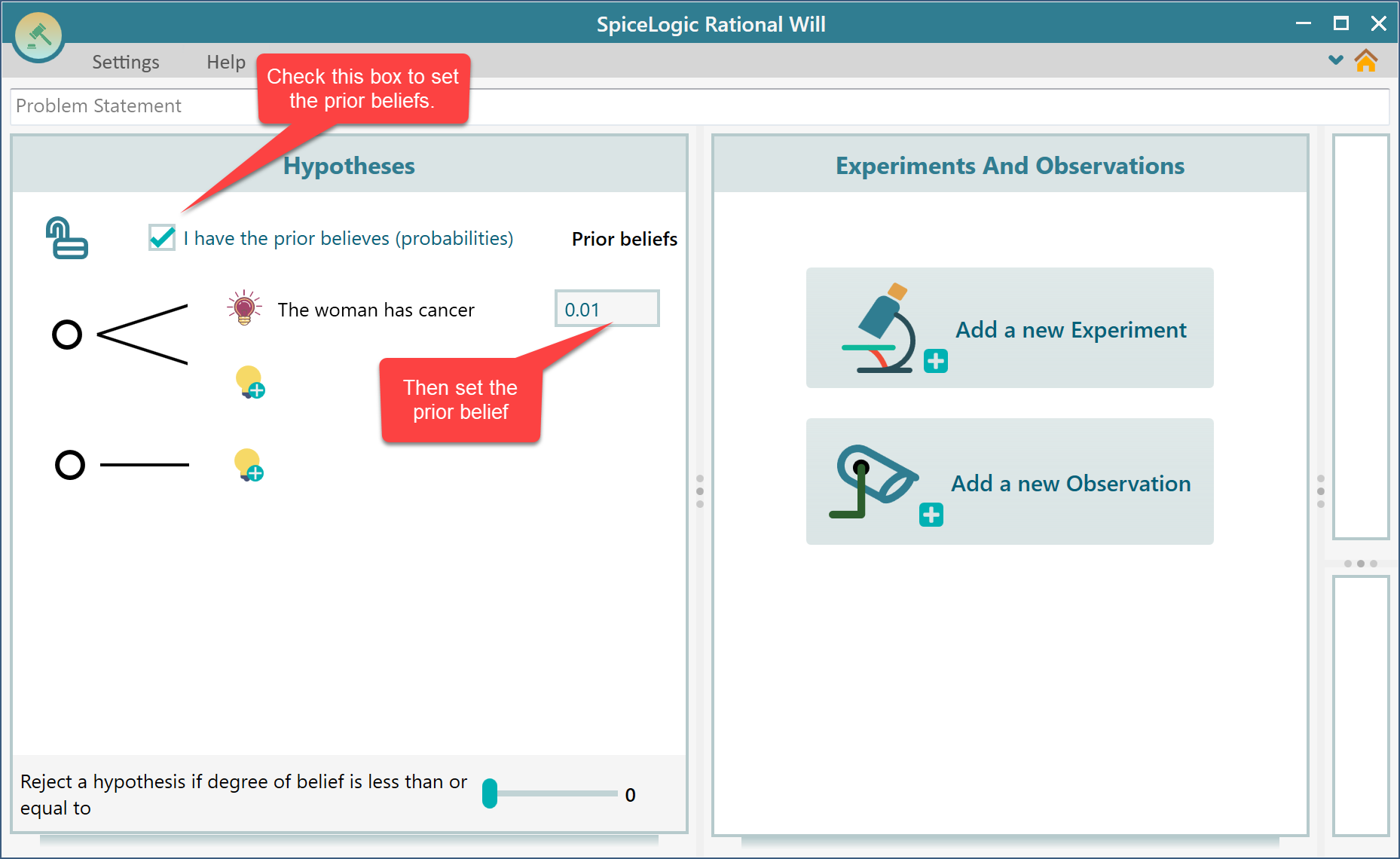
Now, you are In the Bayesian Inference area. Add your Hypothesis that the woman has cancer.

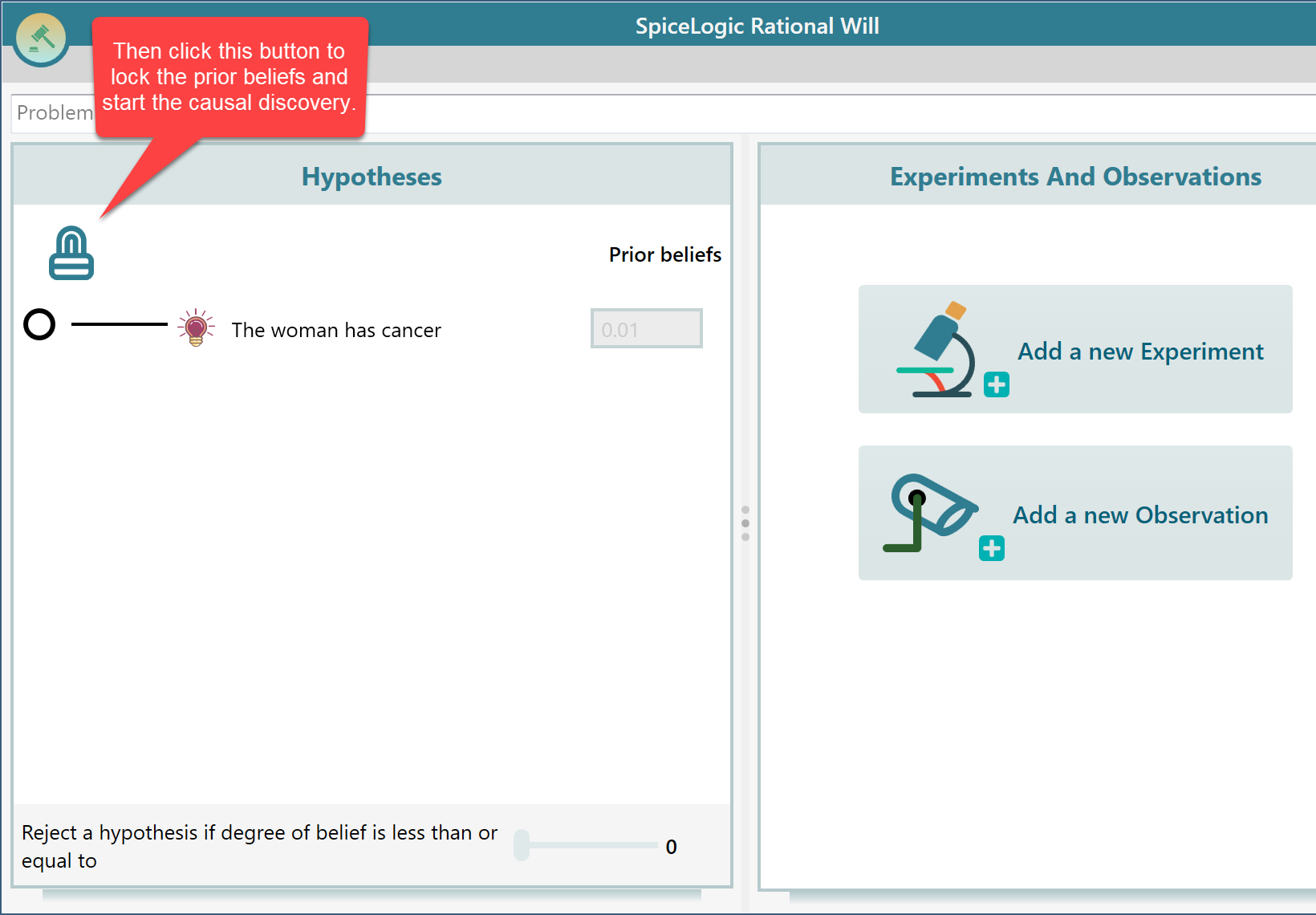
Now, click the Lock button to "Lock" your prior beliefs.

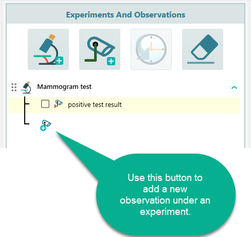
Now, in the Experiments and Observations panel, add a new experiment as "Mammogram test". Under that experiment, add observation "positive test result".

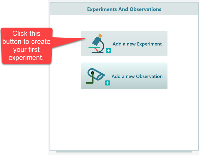
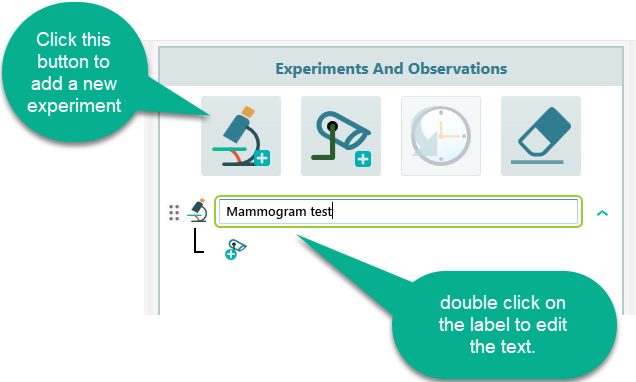
Then, under the added experiment, add a new observation "positive test result".

Finally, concentrate on the Causal Discovery panel.

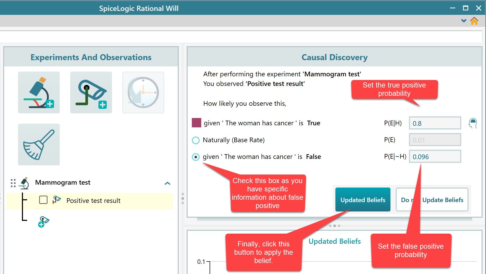
Finding the result

Once you set the True positive and False positive probabilities, click the "Update Beliefs" button. The software will calculate the updated belief based on this information using Bayes Theorem and update the chart of 'Updated Beliefs'. We can see that the probability of the woman having cancer is calculated as 7.76%. This is the new calculated belief that incorporated the base rate in the calculation. Remember that, this is the value we got from our hand calculation.

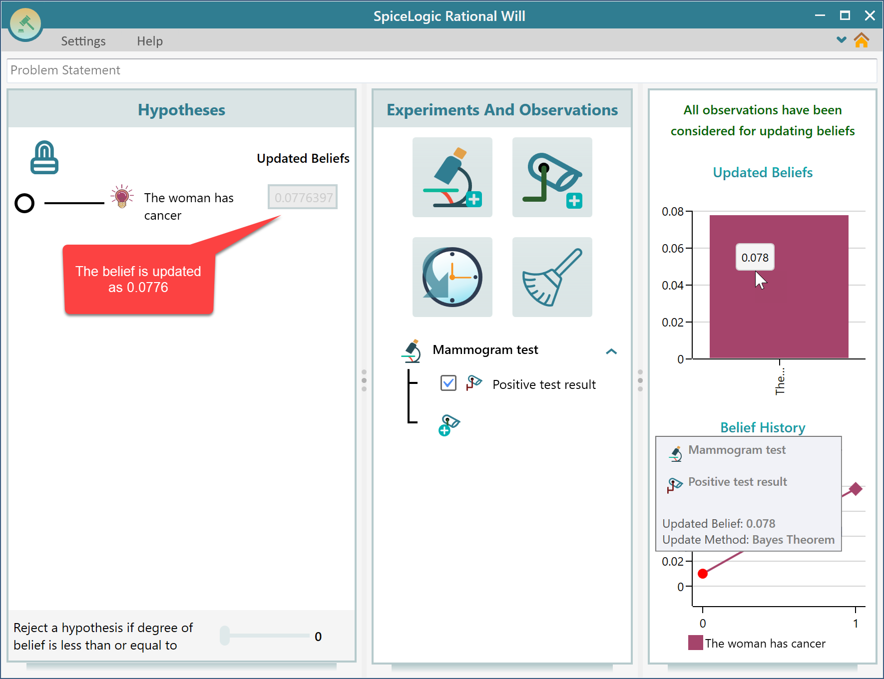
Notice the belief history chart. It shows, how your belief is updated over time, upon evidence. This is an example of Diachronic Interpretation. In the Hypotheses panel, your hypothesis probability is updated as well.

Now, if you observe any new evidence (say, another test result), your prior belief will be this calculated belief, and incorporating this newly calculated belief and your next test result, you can have a new belief. In that way, you can continuously keep updating your beliefs upon pieces of evidence you observe one by one.

If you want to add a new hypothesis or override the hypothesis belief manually, you can click the Lock button to unlock the hypotheses panel, and then change the hypotheses, and then lock again to proceed to causal discovery.

Modeling base rate fallacy in Bayesian Network

You can model the same problem in a Bayesian Network as well. Start the Bayesian Network tool and drag and drop two random variable nodes as shown below. A random variable that represents the woman has cancer. Another random variable represents the positive test result from the mammogram test.

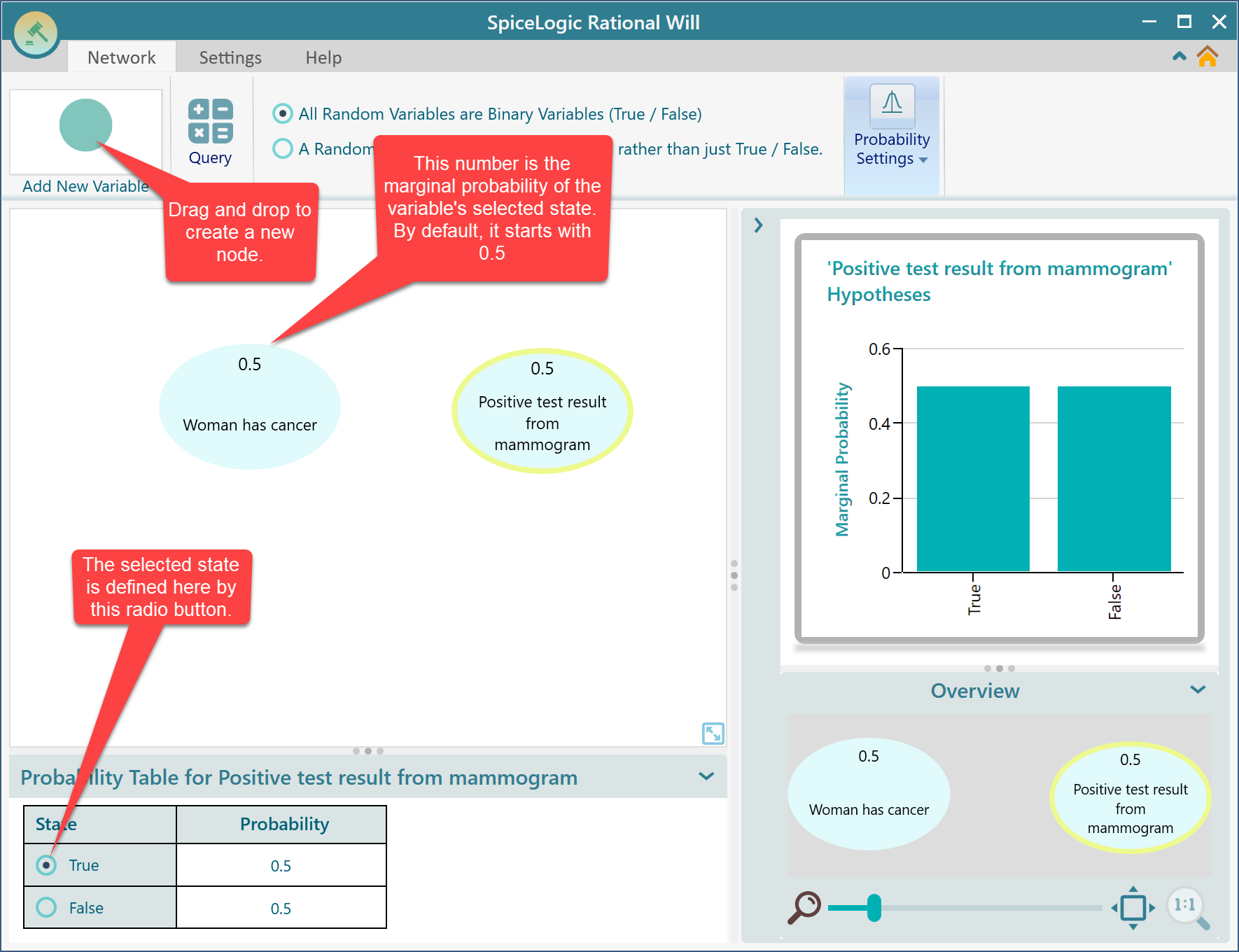
We have a base rate information that 1% of the woman has cancer. So, set the True state variable for 'Woman has cancer' = 0.01. The False state probability will be calculated automatically as 1 - 0.01 = 0.99

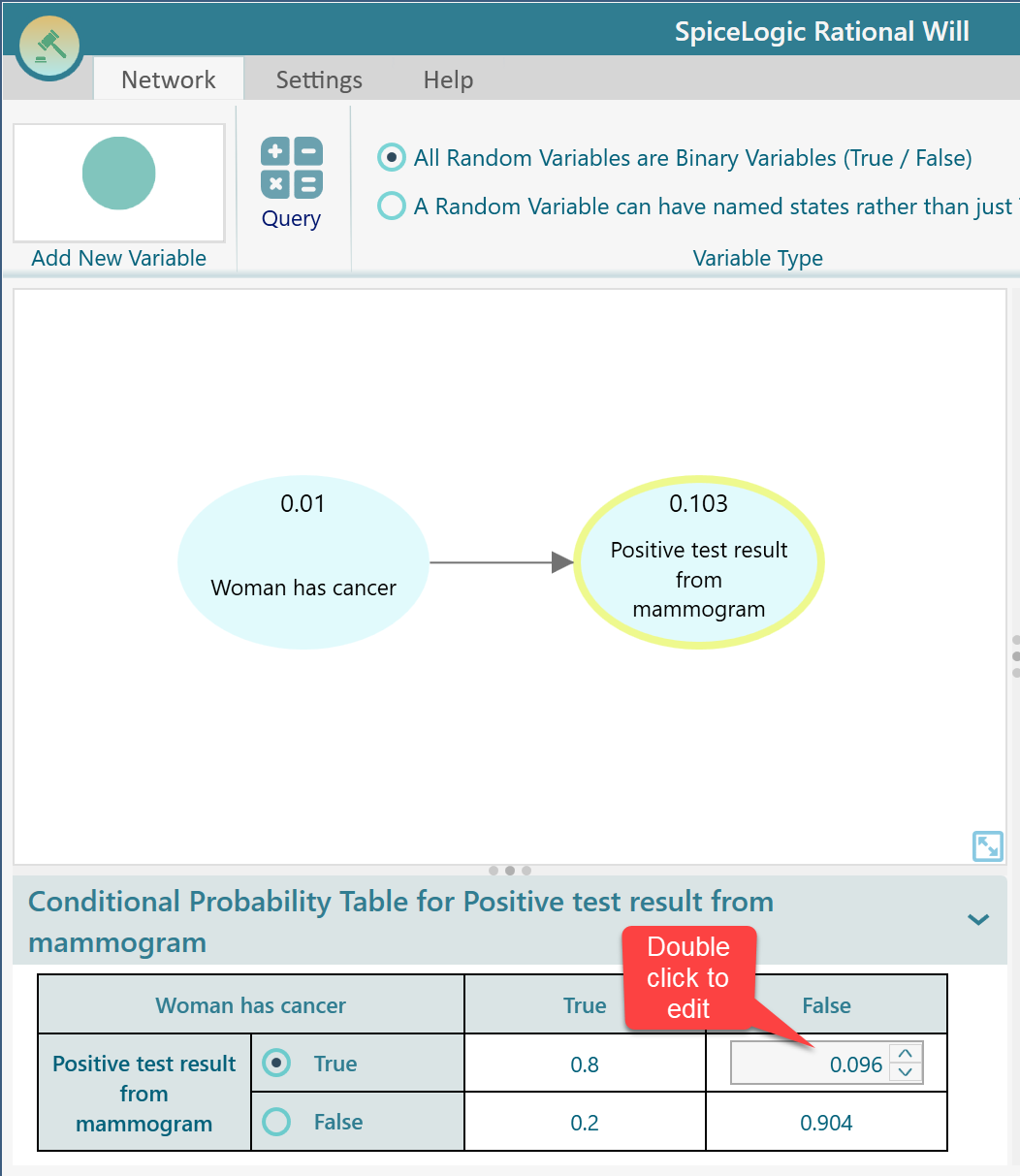
We want to incorporate this base rate information in our judgment. As this base rate information influences the probability of positive test results, draw an arrow connecting the Cancer node to the Positive test result node. Then, select the variable 'Positive test result from mammogram'. You will see the following conditional probability table displayed for this variable. As we know, the mammogram test results positive probability is 0.8 when the woman has cancer. And when the woman does not have cancer, the probability of false-positive is 0.096. So, enter the probabilities accordingly.

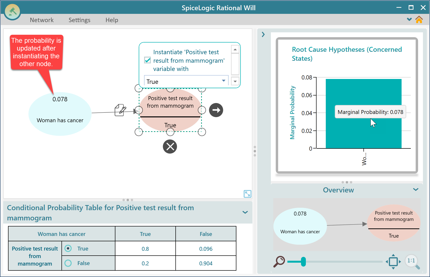
Thus, we have modeled the Bayesian network for this problem. Now, we want to find out what is the probability of the woman having cancer if we observe a positive test result. In order to find that out, select the node "Positive test result" and check the checkbox "Instantiate..."

Notice that, as soon as you instantiate the variable, the "Woman has Cancer" node's marginal probability is displayed as 0.0776. This is the number we got from our hand calculation. So, the diagram confirms that our calculation result was correct. That is the number we were looking for. That means, the Bayesian network calculates the probability of Cancer given that a Positive test result was observed.

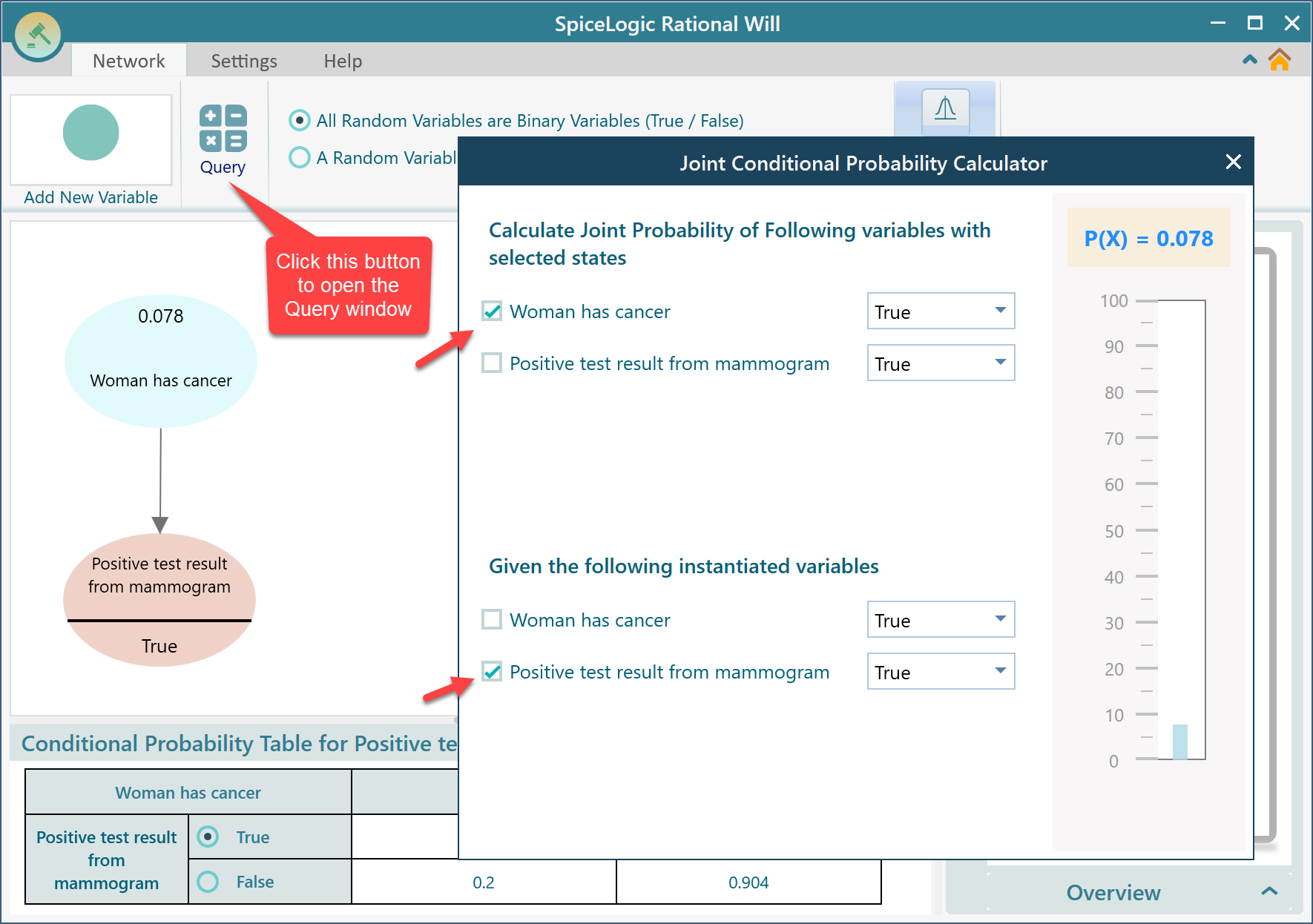
There is another way to find out the probability without instantiating in the diagram. You can open the Query window by clicking the Query button. Then, in the query window, in the top panel, you can check the "Woman has Cancer" and select "True" in the drop-down for Cancer. Then, in the bottom panel, check "positive test result..." and select "True" in the corresponding drop-down. You will see the calculated probability value will be shown as P(X).