Stochastic Dominance
How do you compare two portfolios? The easy answer is to look at the expected value of each one and pick the higher number. That works a lot of the time, but not always. Expected value alone can hide real risk. So you cannot lean on it every time you compare two portfolios, or any two random outcomes.
Why does Stochastic Dominance matter?
It matters most when you do not like risk. A higher average payoff is nice. But if it comes with a real chance of a bad result, a careful person may still walk away from it. Stochastic Dominance gives you a clean way to check that. Say two stocks both have the same average return, but one swings wildly and the other is steady. The averages do not tell you which to trust. Stochastic Dominance does. Look at the simple investment example below.
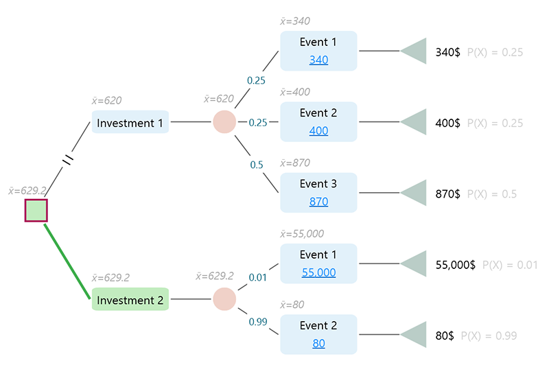
Look at the two investments above. Investment 1 has an expected value of $620. Investment 2 has an expected value of $629.20. If all you care about is the bigger average, you would pick Investment 2. So far, so good.
Now look closer at the actual outcomes and their chances. Investment 2 pays $55,000 with a 1% chance, and only $80 with a 99% chance. Almost every time, you walk away with $80. Investment 1 is far steadier. Even on its worst event, which has a 25% chance, you still get at least $340. Every outcome along the way is solid. Unless you enjoy gambling, you probably would not feel good about choosing Investment 2 over Investment 1, even though Investment 2 has the higher average. Investment 1 just feels safer, and that feeling is real.
So the question becomes this. Is there a math way to tell whether one risky option is genuinely better than another, in a way that rewards consistency? Not just the final average, but something that weighs every outcome together with its probability and tells you which option you can be comfortable with. The answer is Stochastic Dominance.
Here is the catch. Stochastic Dominance will never tell you that a lower-average option beats a higher-average one. If an option has the higher expected value, you still have to look at its risk profile yourself. What Stochastic Dominance does is this. When one option already has the higher expected value, it tells you whether that option is truly better than the other once you account for each outcome and its probability.
So if you find an option with a higher expected value, but it does not stochastically dominate the other option, think twice. That is usually a sign of a gamble. It is a good habit to always check Stochastic Dominance before you make a final call. And remember, this check matters most for someone who wants to avoid risk.
Notations
In the Decision Tree software and Rational Will, Stochastic Dominance is calculated and shown in the Stochastic Dominance Panel. You will see a few short labels there. Here is what each one means.
- FSD = First-Order Stochastic Dominance
- SSD = Second-Order Stochastic Dominance
- TSD = Third-Order Stochastic Dominance
- DD = Deterministic Dominance
- μ σ = Mean-Variance Dominance
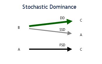
Here is an example view of the Stochastic Dominance Panel, where A, B, and C are different Actions.
First-Order Stochastic Dominance (FSD)
Here is the formal definition from Wikipedia. Random variable A has first-order stochastic dominance over random variable B if, for any outcome x, A gives at least as high a chance of getting at least x as B does, and for some x, A gives a higher chance of getting at least x. In plain terms, no matter what payoff level you pick, A is never worse at reaching it, and at some level A is clearly better. Written out, for all x:

with strict inequality at some x.
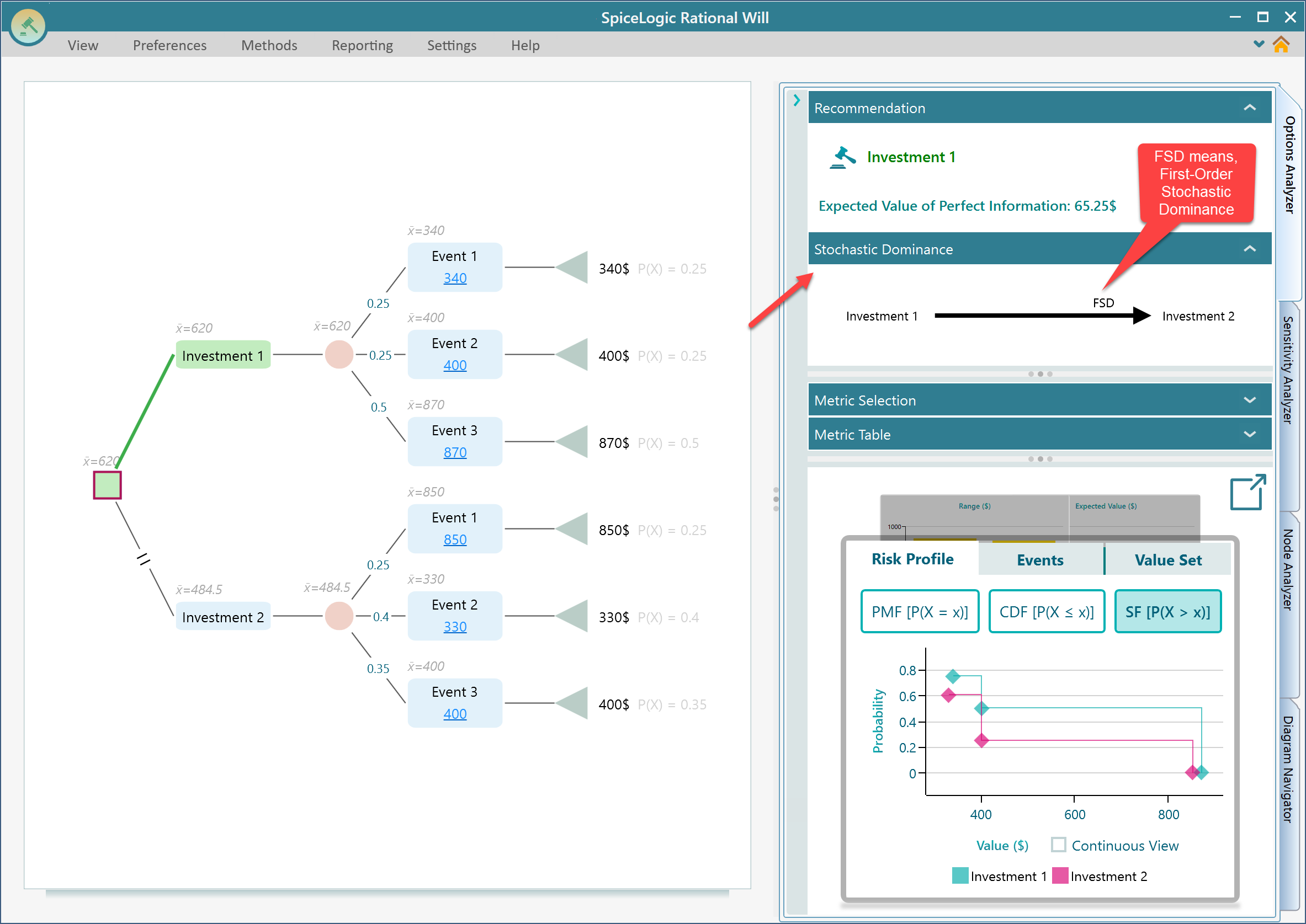
That definition reads better with a picture, so let us walk through an example. Picture two simple investments. At every payoff you might want, the first one gives you at least as good a chance of hitting it, and a better chance at some payoffs. That is the whole idea, and the chart below makes it easy to see. Consider the following decision tree.
Now look at the Risk Profile chart for this decision tree. The Risk Profile chart shows each possible payoff and how likely it is. It is the picture of the gamble behind each option. Here is what you will see.
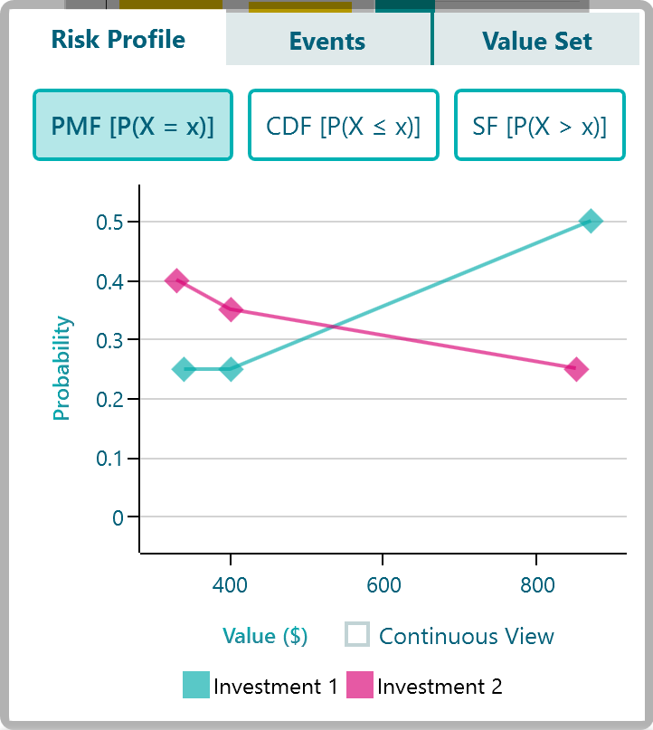
On the Risk Profile chart there is a button labeled SF P (X > x). SF stands for survival function. Click that button to switch the chart to the survival probability view. This view shows, for any payoff you pick, the chance of getting at least that much. That is the view you want for checking first-order dominance, because dominance is all about who has the better chance at every payoff level.
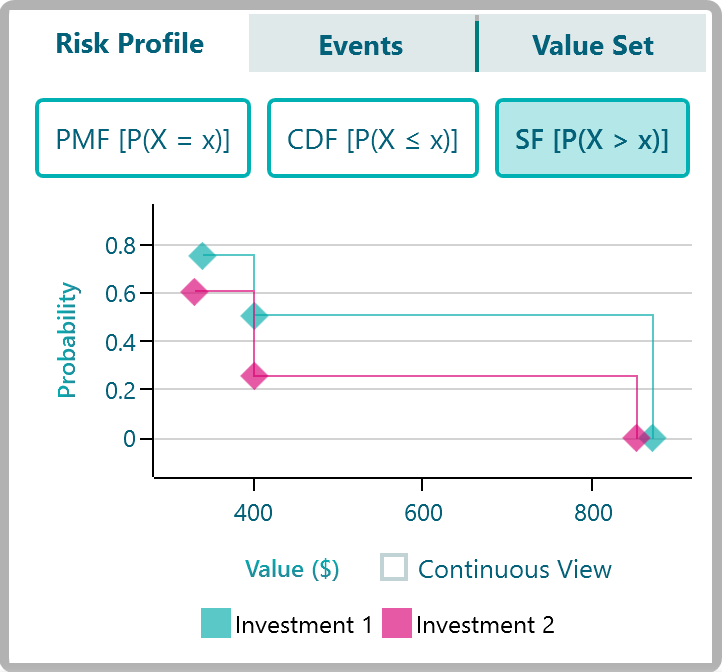
On the Survival Function chart, start around the payoff range of $330 to $340 and read off the chance of getting at least that much. Investment 1 sits at 0.75, and Investment 2 is at 0.6. So in that range, Investment 1 gives you the better chance. Now move to around $400. Both investments can pay $400, but at different odds. The chance of getting at least $400 is 0.5 for Investment 1 and only 0.25 for Investment 2, so Investment 1 wins again. Finally, look at the $850 to $870 range. Here the chance of reaching that payoff is 0% for both.
Now step back and see the pattern. At every payoff level, Investment 1 did at least as well as Investment 2, and often better. So if both options are on the table, an investor can feel more comfortable with Investment 1. Not only because it has the higher expected value, but because it gives a better payoff at any given probability.
That is exactly what first-order stochastic dominance means. Investment 1 outranks Investment 2.
In the SpiceLogic Decision Tree software and Rational Will, you will find a dedicated panel for Stochastic Dominance in the Options Analyzer section. Expand that panel and the dominance is calculated and drawn as a diagram. The label FSD in that panel stands for First-Order Stochastic Dominance.
Second-Order Stochastic Dominance (SSD)
Here is how Wikipedia puts it. For two gambles A and B, gamble A has second-order stochastic dominance over gamble B if A is more predictable, meaning it carries less risk, and has at least as high a mean. Put simply, A is the calmer bet and its average is no worse, so a risk-averse person should still lean toward A. Written out, let:

and

be the cumulative distribution functions of two different investments A and B. Then, for every payoff x:

with strict inequality at some x.
So what does that mean in plain words? Let me put it the way I think about it. With first-order dominance, the winning option had a higher chance of reaching at least every payoff level, top to bottom. That makes the choice easy. But what about a case where the other option, the one that is not the clear winner, actually pays more at some payoff levels? That muddies the decision. The math says you can still prefer the winner up to a point, even when the other option pays more at certain probabilities.
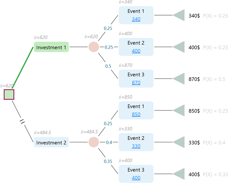
I know, that sounds confusing, so let us make it concrete. Take the same decision tree as before, but raise the payoff of Investment 2, Event 1, from $850 to $1,000. That bumps up the expected value of Investment 2 and makes Investment 1 look a bit less attractive than before. Even so, Investment 1 is still the better option stochastically. This time we say Investment 1 stochastically dominates Investment 2 by the second order.
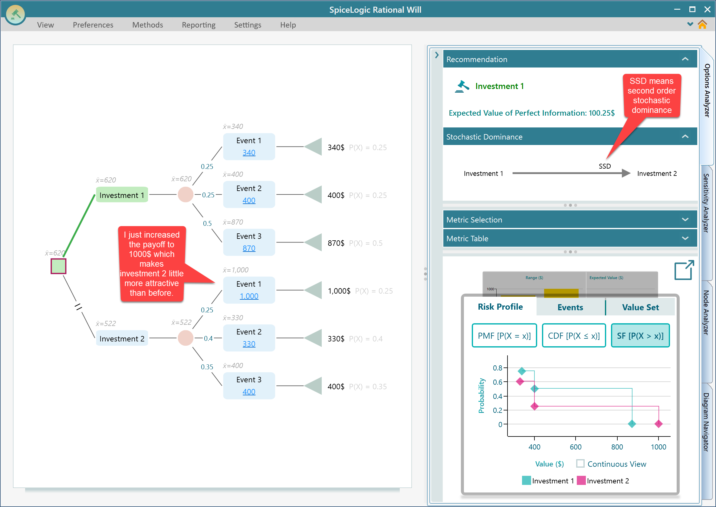
So first-order dominance is stronger than second-order dominance. But if you cannot find an option that wins by the first order, and you find one that wins by the second order instead, that option is still worth considering. Second-order dominance is a real, useful result. It is just a step down from first-order.
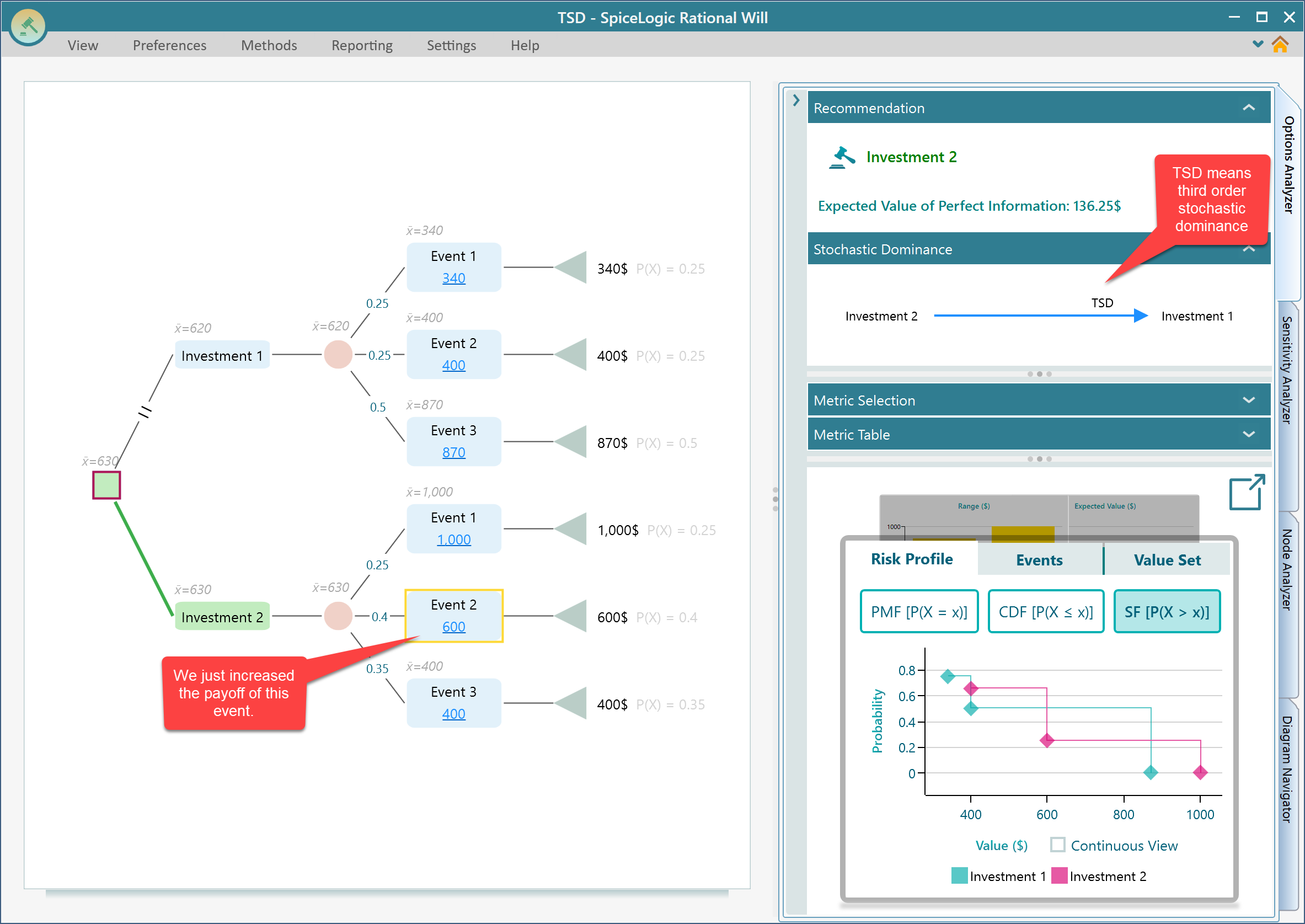
Third-Order Stochastic Dominance (TSD)
The lesson from second-order dominance is that it is a weaker form of first-order dominance. We saw this by raising one payoff of the dominant option, which turned an FSD result into an SSD result. Third-order dominance follows the same idea. It is weaker again than second-order. If you raise yet another payoff of the dominant option from the SSD example, the result drops to third-order dominance, as long as you do not push the payoff of the dominated option too high. We will show this with an example, the same way we did for SSD. But first, here is what Wikipedia says about Third-Order Stochastic Dominance. Let:

and

be the cumulative distribution functions of two different investments A and B. A dominates B in the third order if and only if:


Let us go through an example. Raise another event payoff as shown below. Now Investment 2 ranks higher than Investment 1 on expected value. But because Investment 1 was so much stronger to begin with, that small bump is not enough to make Investment 2 clearly better. It is better, but not by as much as in the FSD or SSD cases. This time, Investment 2 outranks Investment 1 by third-order stochastic dominance.
Other kinds of dominance
The Decision Tree software and Rational Will also show a couple of other kinds of dominance.
- Deterministic Dominance
- Mean-Variance Dominance
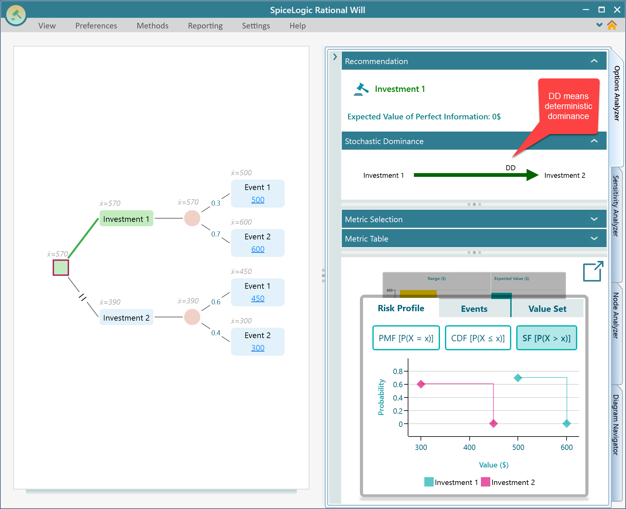
Deterministic Dominance
Deterministic Dominance is the simplest one to understand. If option A's lowest possible payoff is higher than option B's highest possible payoff, then there is nothing to argue about. A beats B every single time, no matter how the chances fall. Even B's best day is worse than A's worst day. Think of one job that pays at least $5,000 a month no matter what, against another that tops out at $4,000 on its best month. The first one wins before you even look at the odds. That is Deterministic Dominance. Here is an example.
Mean-Variance Dominance
Quite often there is no stochastic dominance between two random outcomes at all. When that happens, the SpiceLogic Decision Tree software and Rational Will look for another way to tell whether one set of uncertainties is better than the other. That is Mean-Variance Dominance. Think of a lottery or any big jackpot game. The payoff has a huge standard deviation, and only people who enjoy gambling go for an outcome that swings that wildly. When you compare two options, the one with the lower standard deviation gives you a steadier, more predictable result. So suppose option A has a higher expected value than option B, and at the same time A has a lower standard deviation than B. Then A is clearly the better choice. Not only because its average is higher, but because its outcomes vary less. This is shown as Mean-Variance Dominance in the software, like the example below.
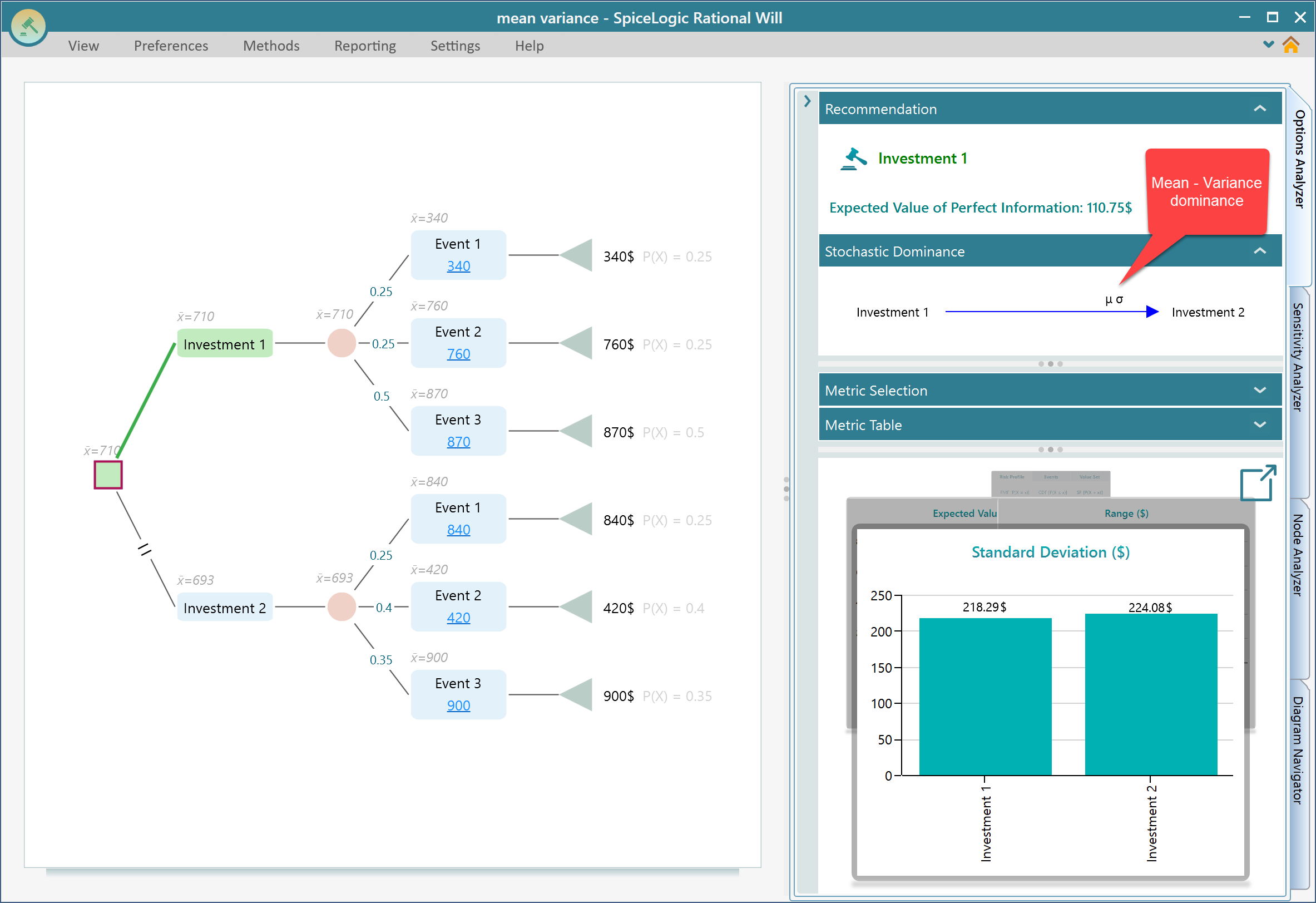
In the screenshot above, Investment 1 has an expected value of $710 and a standard deviation of $218.29. Investment 2 has an expected value of $693 and a standard deviation of $224.08. So Investment 1 has the higher average and the lower spread, which means Investment 1 dominates Investment 2 by mean-variance.
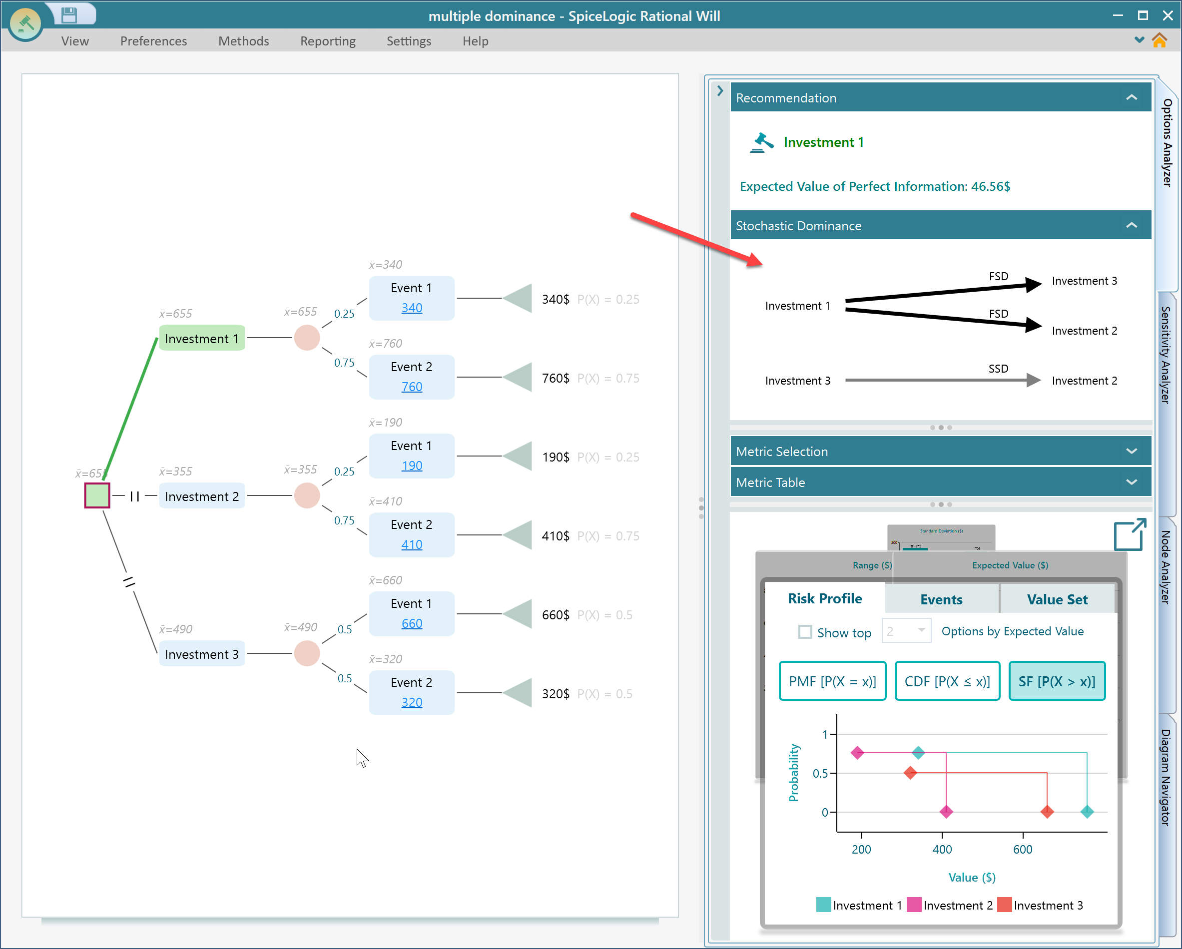
Multiple kinds of dominance in the same decision tree
When you have more than two options, things get interesting. One option might dominate a second by first-order stochastic dominance and dominate a third by second-order stochastic dominance, all at once. It helps to see which option beats which, and by what degree. The SpiceLogic Decision Tree software and Rational Will show you all of this in a single dominance diagram, like the one below.